To a certain extent, coding matrices in frequentist inference are arbitrary. We might choose a certain coding to make inference for hypotheses straightforward in the context of the model parameterisation. For example (see vignette Venables 2018), assuming \(p\) cell means of interest \(\mu\), we could begin with the incidence matrix \[ X = \begin{pmatrix} \mathbf 1_{n_1} & 0 & \cdots & 0 \\ 0 & \mathbf 1_{n_2} & \cdots & 0 \\ \vdots & \vdots & \ddots & \vdots \\ 0 & 0 & \cdots & \mathbf 1_{n_p} \end{pmatrix} \] with linear predictor \(\eta = X\mu\). From this we can transform our design matrix into any other linear coding, \(C = B^{-1}\), by using appropriate invertible transformation matrices such that \(\beta = C\mu\) so that \(\eta = XB\beta\). We can essentially always parameterise the model in terms of cell means and work out what we want later.

In Bayesian analyses, if careful consideration is not given to priors, our model parameterisation may influences our inferences in unintended ways. Setting by some kind of default specification may not always reflect the prior information we wish to encode, and without careful thought, may imply some undesired model characteristics.

For example, suppose we were undertaking a three arm trial to compare the effects of three independent treatments. We are interested in making a decision regarding every treatment comparison. By default, we might assume a logistic regression model and code in terms of treatment effects \[ \begin{aligned} \eta_i &= \beta_0 + \beta_1 x_{i1} + \beta_2 x_{i2} \\ \beta &\sim N(0, \sigma^2 I_3) \\ y_i|\beta &\sim \text{Ber}(\text{logit}^{-1}\eta_i). \end{aligned} \] We are then interested in \(\mathbb P_{\beta|Y}(\beta_1 > 0), \mathbb P_{\beta|Y}(\beta_2 > 0)\), and \(\mathbb P_{\beta|Y}(\beta_2 - \beta_1 > 0)\).

Alternatively, we might have decided to parameterise in terms of cell means \[ \begin{aligned} \eta_i &= \beta^C_0 x_{i0} + \beta^C_1 x_{i1} + \beta^C_2 x_{i2} \\ \beta^C &\sim N(0, \sigma^2 I_3) \\ y_i|\beta^C &\sim \text{Ber}(\text{logit}^{-1}\eta_i). \end{aligned} \] We are then interested in \(\mathbb P_{\beta^C|Y}(\beta^C_1 - \beta_0^C > 0), \mathbb P_{\beta^C|Y}(\beta^C_2 - \beta_1^C > 0)\), and \(\mathbb P_{\beta^C|Y}(\beta_2 - \beta_1 > 0)\).

Suppose we observe sample sizes \(n = (20, 20, 20)\) within each group and successes \(y = (4, 10, 16)\) and set our prior scale to \(\sigma=1\). From the observed data and given our priors, we might think it reasonable that our posterior evidence that treatment 2 is better than treatment 1 should be equivalent to our posterior evidence that treatment 3 is better than treatment 2, given that our observations for treatment 1 and 3 are equidistant from the treatment 2 response which is exactly on 0.5. However, our prior information would not lead us to this conclusion.

data {
  int<lower=1> N;
  int<lower=1> P;
  int<lower=0> n[N];
  int<lower=0> y[N];
  matrix[N, P] X;
  vector[N] mu0;
  matrix[P, P] sigma0;
}
parameters {
  vector[P] beta;
}
model {
  vector[N] eta;
  eta = X * beta;
  target += multi_normal_lpdf(beta | mu0, sigma0);
  target += binomial_logit_lpmf(y | n, eta);
}

library(rstan)
n <- 2*rep(10, 3)
y <- 2*c(2, 5, 8)
X1 <- matrix(c(1, 1, 1, 0, 1, 0, 0, 0, 1), 3, 3)
X2 <- matrix(c(1, 0, 0, 0, 1, 0, 0, 0, 1), 3, 3)
dat1 <- list(N = 3, P = 3, X = X1, n = n, y = y, mu0 = rep(0, 3), sigma0 = diag(1, 3))
dat2 <- list(N = 3, P = 3, X = X2, n = n, y = y, mu0 = rep(0, 3), sigma0 = diag(1, 3))
m_out1 <- sampling(log_reg, data = dat1, refresh = 0, iter = 2e4)
m_out2 <- sampling(log_reg, data = dat2, refresh = 0, iter = 2e4)
m_draws1 <- as.matrix(m_out1)[, 1:3]
m_draws2 <- as.matrix(m_out2)[, 1:3]

Figure 1 presents our posterior densities of the treatment differences under the effect coding model and the cell means model.

nice_par(mfrow = c(2, 2))
plot(density(m_draws1[, 2], n = 1e3), 
     main = "Effect coding", 
     xlab = "Estimated treatment difference",
     xlim = c(-2, 4), ylim = c(0, 0.8))
lines(density(m_draws1[, 3] - m_draws1[, 2], n = 1e3), col = "red")
legend("topleft", legend = c("2 vs 1", "3 vs 2"), lty = c(1, 1), 
       col = c(1, "red"), bty = 'n')
plot(density(m_draws2[, 2] - m_draws2[, 1], n = 1e3), 
     main = "Cell coding", 
     xlab = "Estimated treatment difference",
     xlim = c(-2, 4), ylim = c(0, 0.8))
lines(density(m_draws2[, 3] - m_draws2[, 2], n = 1e3), col = "red")
legend("topleft", legend = c("2 vs 1", "3 vs 2"), lty = c(1, 1), 
       col = c(1, "red"), bty = 'n')

plot(m_draws1[, 2], m_draws1[, 3] - m_draws1[, 2], 
     col = rgb(0, 0, 0, alpha = 0.025), pch = 19,
     xlab = "2 vs 1", ylab = "3 vs 2", xlim = c(-2, 4), ylim = c(-2, 4))
plot(m_draws2[, 2] - m_draws2[, 1], m_draws2[, 3] - m_draws2[, 2], 
     col = rgb(0, 0, 0, alpha = 0.025), pch = 19, 
     xlab = "2 vs 1", ylab = "3 vs 2", xlim = c(-2, 4), ylim = c(-2, 4))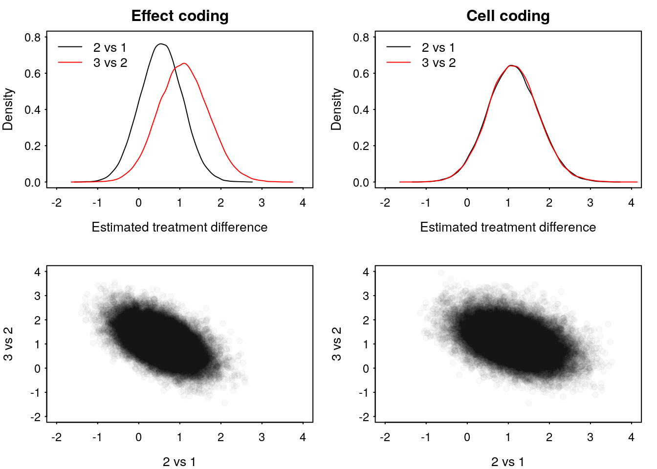

Figure 1: Comparison between effect and cell coding priors on posterior densities.

cat("Effect coding\n")
c("Prob(Trt 2 > Trt 1)" = mean(m_draws1[, 2] > 0), 
  "Prob(Trt 3 > Trt 2)" = mean(m_draws1[, 3] - m_draws1[, 2] > 0))
cat("Cell coding\n")
c("Prob(Trt 2 > Trt 1)" = mean(m_draws2[, 2] - m_draws2[, 1] > 0),
  "Prob(Trt 3 > Trt 2)" = mean(m_draws2[, 3] - m_draws2[, 2] > 0))

Effect coding
Prob(Trt 2 > Trt 1) Prob(Trt 3 > Trt 2) 
           0.854175            0.965675 
Cell coding
Prob(Trt 2 > Trt 1) Prob(Trt 3 > Trt 2) 
           0.967250            0.966525 

If we were making a threshold based decision dependent on a posterior probability of 0.95 then we might conclude sufficient evidence to say treatment 3 is better than 2, but not that treatment 2 is better than 1, even though the data provides the same evidence.

What happened? Our prior specification on the effects parameterisation implies different prior scales on the treatment comparisons \[ \begin{aligned} \beta &\sim N\left(0, \sigma^2 I_3\right) \\ \implies \begin{pmatrix} \beta_1 \\ \beta_2 - \beta_1 \end{pmatrix} &\sim N\left(0, \begin{pmatrix} \sigma^2 & -\sigma^2 \\ -\sigma^2 & 2\sigma^2 \end{pmatrix}\right). \end{aligned} \] So, apriori, we have specified that we are more confident that the difference between treatment 2 and 1 is close to zero then we are that the difference between treatment 3 and 2 is close to zero. Therefore, the posterior density of the treatment difference between 2 and 1 is relatively less influenced by the data.

Under the cell means prior we implicitly set equivalent scales. \[ \begin{aligned} \beta^C &\sim N\left(0, \sigma^2 I_3\right) \\ \implies \begin{pmatrix} \beta^C_1 - \beta_0^C \\ \beta^C_2 - \beta^C_1 \end{pmatrix} &\sim N\left(0, \begin{pmatrix} 2\sigma^2 & -\sigma^2 \\ -\sigma^2 & 2\sigma^2 \end{pmatrix}\right). \end{aligned} \]

Of course, we can get equivalent results between the two codings just by choosing appropriate priors given the parameterisation. The problem only occurs if we didn’t put any thought into how we parameterised the model or our priors and what it is we are trying to infer. Thus, our priors fail to reflect our true prior information or assumptions.

In some instances we may want to set different scales on the comparisons, for example, if treatment 1 was a standard of care and treatment 2 and 3 were standard of care plus an additional new treatment, we might believe that apriori we are more informed about the comparisons between treatments 1 and 2 and treatments 1 and 3 than we are about comparisons between treatment 2 and 3 because the first two involve only one new treatment whereas the third involves both new treatments. We should then specify the prior scales appropriately to reflect this information.

The takeaway is don’t specify a prior without thinking about what we want to infer and how our specified prior might influence those inferences.

References

Venables, Bill. 2018. CodingMatrices: Alternative Factor Coding Matrices for Linear Model Formulae. https://CRAN.R-project.org/package=codingMatrices.