Background
Previously, I had worked through derivations of variational approximations for a linear regression model and proportional hazards exponential model with right-censoring. This post works through approximations for logistic regression models.
Some general references on variational approximations for logistic regression are Murphy (2012), Nolan and Wand (2017), and Wand (2017).
Recall the evidence lower bound (ELBO) is given by \[ \begin{aligned} \ln p(y|\theta) &\geq \mathcal{L}(y|\theta;q) \\ &= \mathbb E_q[\ln p(y,\theta) - \ln q(\theta)] \\ &= \mathbb E_q[\ln p(y|\theta)] + \mathbb E_q[\ln p(\theta)] + \mathbb H_q[\theta]. \end{aligned} \]
The model we are interested in is \[ \begin{aligned} y|\beta &\sim Ber(\text{expit}(X\beta)) \\ \beta &\sim N(\mu_0,\Sigma_0), \end{aligned} \] where \(\text{expit(x)} = \text{logit}^{-1}(x) = (1 + e^{-x})^{-1}\).
The values \(\mathbb E_q[\ln p(\theta)]\) and \(\mathbb H_q[\theta]\) are known \[ \begin{aligned} \mathbb E_q[\ln p(\beta)] &= -\frac{1}{2}\left\{d\ln(2\pi) + \ln|\Sigma_0| + \mathbb E[(\beta - \mu_0)^\top\Sigma_0^{-1}(\beta-\mu_0)]\right\} \\ &= -\frac{1}{2}\left\{d\ln(2\pi)+\ln|\Sigma_0| + (\mu_\beta-\mu_0)^\top\Sigma_0^{-1}(\mu_\beta-\mu_0) + \text{tr}(\Sigma_0^{-1}\Sigma_\beta)\right\} \\ \mathbb H_q[\beta] &= \frac{1}{2}\left[d(1 + \ln(2\pi)) + \ln|\Sigma_\beta|\right] \\ \mathbb E_q[\ln p(\beta)] + \mathbb H_q[\beta] &= \frac{d}{2} + \frac{1}{2}\ln|\Sigma_\beta|-\frac{1}{2}\ln|\Sigma_0|-\frac{1}{2}(\mu_\beta-\mu_0)^\top\Sigma_0^{-1}(\mu_\beta-\mu_0) - \frac{1}{2}\text{tr}(\Sigma_0^{-1}\Sigma_\beta) \end{aligned} \] where \(\mathbb E_q[\beta] = \mu_\beta\) and \(\Sigma_\beta = \mathbb V_q[\beta]\).
From the model likelihood we have \[ \ln p(y|\beta) = y^\top X\beta - 1^\top\ln(1 + \exp(X\beta)) \] which presents the challenge of finding \[ \mathbb E_q[\ln(1 + \exp(\eta_i))] \] under a given \(q\) where \(\eta_i = x_i^\top\beta\). Generally, we will assume that \(q(\beta) = N(\beta|\mu_\beta,\Sigma_\beta)\), that is, the approximating family is normal distributions.
There are many ways we might deal with the intractability of this expectation. Common approaches are to utilise an approximation to the log-sum-exp term providing a new lower bound and simpler expectation, or to work with the integral directly utilising quadrature rules. In this post I will focus on approximation bounds and look at approaches using quadrature in the future.
Approximation Bounds
The approach is to replace the intractable bound by one which is easier to work with. Generally, this involves using a new bound such that \[ \ln p(y|\theta) \geq \ln\tilde p(y|\theta). \] by applying a lower bound on the value of \(-\ln(1 + \exp(\eta))\).
All the fixed-point updates that follow are a result of general optimisation methods. Details can be found in Rhode and Wand (2016).
Bohning
Böhning and Lindsay (1988) show how to adjust Newton-Raphson method to attain monotonical convergence by applying a lower-bound on the Hessian which is equivalent to a quadratic approximation change in a function relative to the point of Taylor series expansion. Böhning (1992) gives an application of this bound to estimation in multinomial logistic regression.
We perform a Taylor series expansion of the log-sum-exp function around a point \(\psi_i\). \[ \begin{aligned} \ln(1 + e^{\eta_i}) &= \ln(1 + e^{\psi_i}) + (\eta_i - \psi_i)g(\psi_i)+\frac{1}{2}(\eta_i-\psi_i)^2H(\psi_i) \\ g(\psi_i) = \frac{d}{d\psi_i}\ln(1 + e^{\psi_i}) &= \text{expit}(\psi_i) = \exp(\psi_i - \ln(1 + e^{\psi_i})) \\ H(\psi_i) = \frac{d^2}{d\psi_i^2}\ln(1 + e^{\psi_i}) &= \text{expit}(\psi_i)(1 - \text{expit}(\psi_i)) \end{aligned} \] An upper bound on the function can be obtained by replacing \(H(\psi_i)\) by the upper bound 1/4 (the value of \(\text{expit}(\eta)(1-\text{expit}(\eta))\leq1/4\) being maximal when both values are \(1/2\)).
The result is a quadratic bound \[ \begin{aligned} \ln(1 + e^\eta) &\leq \frac{1}{2}a\eta^2-b(\psi)\eta+c(\psi)\\ &= BB(\psi, x) \\ a &= \frac{1}{4} \\ b(\psi) &= a\psi - \text{expit}(\psi) \\ c(\psi) &= \frac{1}{2}a\psi^2 - \text{expit}(\psi)\psi + \ln(1 + e^\psi). \end{aligned} \]
Figure 1 shows the Bohning bound compared to the log-sum-exp function for various fixed \(x\) while varying \(\psi\). Figure 2 shows the bound on the sigmoid function itself as a function of \(x\) for various fixed \(\psi\).
a_psi <- 1/4
b_psi <- function(psi) psi/4 - plogis(psi)
c_psi <- function(psi) psi^2/8 - psi*plogis(psi) + log(1 + exp(psi))
bb_bound <- function(psi, x) {
  1/2*a_psi*x^2 - b_psi(psi)*x + c_psi(psi)
}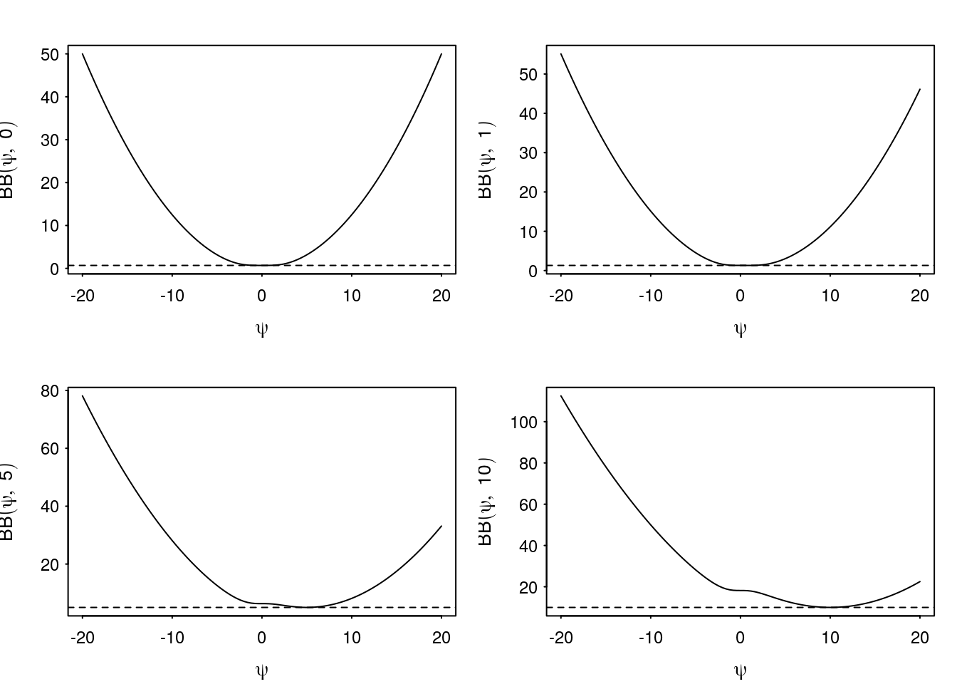
Figure 1: Examples of the Bohning bound as a function of \(\psi\) for fixed \(x\).
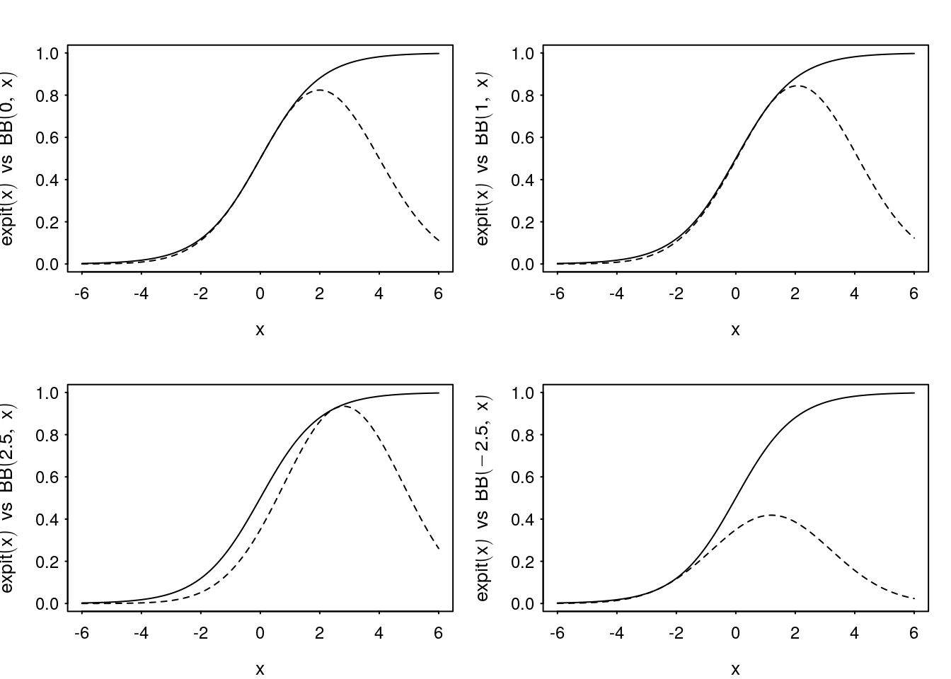
Figure 2: Examples of Bohning quadratic bound for \(\text{expit}(x)\) as a function of \(x\) for varying \(\psi\).
Substituting the bound for the log-sum-exp function we find \[ \sum_{i=1}^n \mathbb E_q\left[\frac{1}{2}ax_i^\top\beta\beta^\top x_i^\top-b(\psi_i)x_i^\top\beta+c(\psi_i)\right] =\quad \sum_{i=1}^n \frac{1}{2}ax_i^\top\mathbb E_q[\beta\beta^\top]x_i-b(\psi_i)x_i^\top\mu_\beta+c(\psi_i). \] To optimise this new variational parameter we find \[ \mathsf{D}_{\psi_i}\mathcal{L}(q) = -\left(\frac{1}{4}-\frac{\partial}{\partial\psi_i}\text{expit}(\psi_i)\right)x_i^\top\mu_\beta+\left(\frac{1}{4}-\frac{\partial}{\partial\psi_i}\text{expit}(\psi_i)\right)\psi_i \] which can only equal zero if \(\psi_i=x_i^\top\mu_\beta\).
Additionally, \[ \begin{aligned} \mathsf{D}_{\mu_\beta}\mathcal{L}(q) &= X^\top y-\frac{1}{4}X^\top X\mu_\beta + X^\top b(\psi) - \Sigma_0^{-1}(\mu_\beta-\mu_0) \\ \mathsf{H}_{\mu_\beta}\mathcal{L}(q) &= -\frac{1}{4}X^\top X-\Sigma_0^{-1}\mu_\beta \end{aligned} \] from which we arrive at the iterative updates \[ \begin{cases} \psi &\leftarrow X\mu_\beta \\ \mu_\beta &\leftarrow \Sigma_\beta\left(X^\top(y+b(\psi))+\Sigma_0^{-1}\mu_0\right) \\ \Sigma_\beta &\leftarrow \left(\Sigma_0+\frac{X^\top X}{4}\right)^{-1} \end{cases} \] and evidence lower bound \[ \begin{aligned} \mathcal{L}(q;\psi) &= \frac{d}{2} + \frac{1}{2}\ln|\Sigma_\beta|-\frac{1}{2}\ln|\Sigma_0|-\frac{1}{2}(\mu_\beta-\mu_0)^\top\Sigma_0^{-1}(\mu_\beta-\mu_0) - \frac{1}{2}\text{tr}(\Sigma_0^{-1}\Sigma_\beta) \\ &\quad y^\top X\mu_\beta-\frac{1}{8}\text{tr}\left(X(\Sigma + \mu_\beta\mu_\beta^\top)X^\top \right)+b(\psi)^\top X\mu_\beta-1^\top c(\psi). \end{aligned} \]
Jaakkola-Jordan
The Jaakkola-Jordan approximation is based on the following arguments. They (Jaakkola and Jordan 2000) first symmetrise the function of interest \[ -\ln(1 + e^x) = -x/2-\ln\left(e^{x/2}+e^{-x/2}\right) \] and then lower bound the function \(f(x) = -\ln\left(e^{x/2}+e^{-x/2}\right)\) (which is convex) by a first order Taylor expansion on \(x^2\) \[ -\ln\left(e^{x/2}+e^{-x/2}\right) = f(x) \geq f(\xi) + \frac{\partial f(\xi)}{\partial (\xi^2)}(x^2-\xi^2) = \frac{\xi}{2} - \ln(1 + e^\xi) - \frac{\tanh(\xi/2)}{4\xi}(x^2-\xi^2). \] with exactness when \(x^2 = \xi^2\).
Therefore, we have \[ \begin{aligned} \ln(1 + e^x) &= \frac{x}{2} + \ln\left(e^{x/2}+e^{-x/2}\right)\\ &\leq \frac{x}{2} - \frac{\xi}{2} + \ln(1 + e^\xi) + \frac{\tanh(\xi/2)}{4\xi}(x^2-\xi^2) \\ \text{JJ}(\xi,x) &= \frac{1}{2}A(\xi)x^2-Bx+C(\xi) \\ A(\xi) &= 2\frac{\tanh(\xi/2)}{4\xi}\\ B &= -\frac{1}{2} \\ C(\xi) &= - \frac{\xi\tanh(\xi/2)}{4}-\frac{\xi}{2} + \ln(1 + e^\xi), \end{aligned} \] and for each \(x\in\mathbb R\) there exists a \(\xi\in\mathbb R\) such that equality is attained.
The bound is undefined at and symmetric about \(\xi=0\) (Figure 3). Due to the symmetry and approximation attains a tight bound at both \(\xi=\pm\xi^\star\) for a solution \(\xi^\star\) (Figure 4). Compare this to the previous Bohning approximation which only attains a tight bound for one value of \(\psi\).
A_xi <- function(xi) 2*tanh(xi/2)/(4*xi)
B_xi <- -1/2
C_xi <- function(xi) -xi/2 + log(1 + exp(xi)) - xi*tanh(xi/2)/4
jj_bound <- function(xi, x) {
  A_xi(xi)/2*x^2 - B_xi*x + C_xi(xi)
}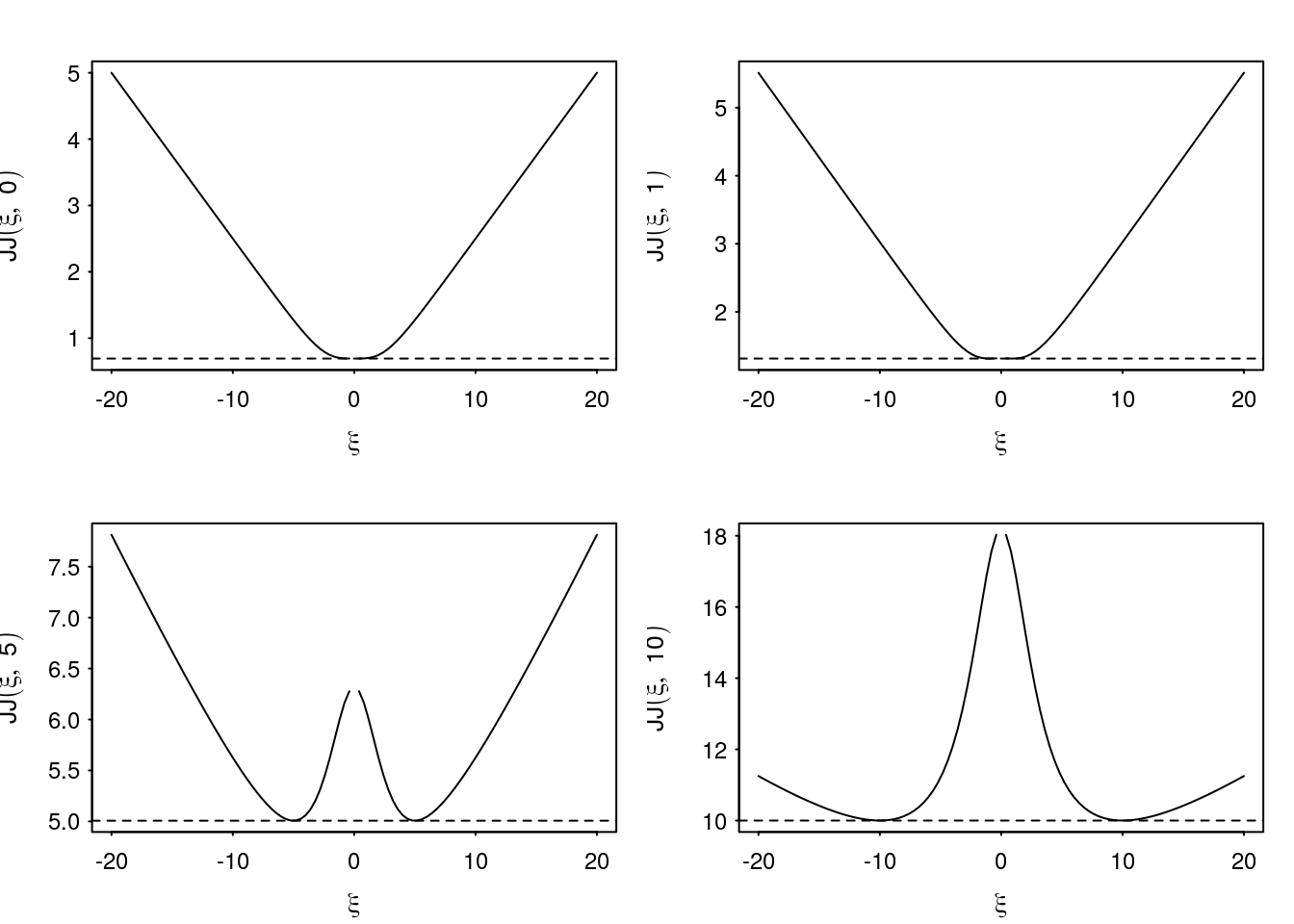
Figure 3: Examples of the Jaakkola-Jordan bound as a function of \(\xi\) for fixed \(x\).
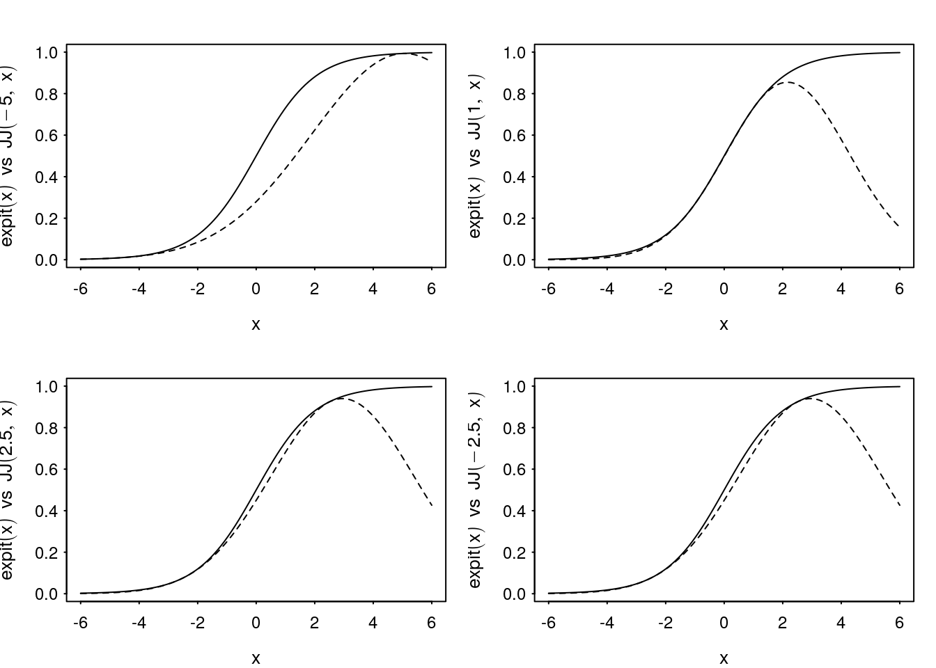
Figure 4: Examples of Jaakkola-Jordan quadratic bound for \(\text{expit}(x)\) as a function of \(x\) for varying \(\xi\).
Using this new bound on \(\ln p(y|\beta)\), the function to maximise depends on the new bound \[ \begin{aligned} \mathbb E_q[\ln p(y|\beta)] &= \mathbb E_q[y^\top X\beta] - 1^\top\mathbb E_q[\ln(1 + \exp(X\beta)]\\ &\geq \mathbb E_q[y^\top X\beta] - \mathbb E_q\left[-\frac{1}{2}X\beta + \beta^\top X^\top\text{diag}\left(\frac{\tanh(\xi/2)}{4\xi}\right)X\beta+1^\top C(\xi)\right]\\ &= \left(y-\frac{1}{2}1\right)^\top X\mu_\beta - \mathbb E_q\left[\beta^\top X^\top\text{diag}\left(\frac{\tanh(\xi/2)}{4\xi}\right)X\beta\right]+1^\top C(\xi) \end{aligned} \]
We have \[ \mathbb E_q\left[\beta^\top X^\top\text{diag}\left(\frac{\tanh(\xi/2)}{4\xi}\right)X\beta\right] = \text{tr}\left(\mathbb E_q[\beta\beta^\top]X^\top \text{diag}\left(\frac{\tanh(\xi/2)}{4\xi}\right)X\right) \] If we want to optimise with respect to \(\xi\) we find that as a function of \(\xi\), \[ \begin{aligned} \mathsf{D}_{\xi_i}\left[\frac{\xi_i}{2} - \ln(1 + e^{\xi_i}) - \frac{\tanh(\xi_i/2)}{4\xi_i}\left(x_i^\top\mathbb E_q[\beta\beta^\top]x_i-\xi_i^2\right)\right] &= \mathsf D_{\xi_i}\left[\frac{\tanh(\xi_i/2)}{4\xi_i}\right](x_i^\top\mathbb E_q[\beta\beta^\top]x_i-\xi_i^2) \end{aligned} \] which implies (due to monotonicity of the required derivative and symmetry of the bound about \(\xi_i=0\)) the update \[ \xi \leftarrow \sqrt{\text{diag}\left(X \left\{\mathbb V[\beta] + \mathbb E[\beta]\mathbb E[\beta]^\top\right\}X^\top\right)} \]
Additionally, \[ \begin{aligned} \mathsf{D}_{\mu_\beta} &= \left(y - \frac{1}{2}1\right)^\top X - \left(X^\top\text{diag}\left(\frac{\tanh(\xi/2)}{2\xi}\right)X\right)\mu_\beta -\Sigma_0^{-1}\mu_\beta + \Sigma_0^{-1}\mu_0 \\ \mathsf{H}_{\mu_\beta} &= -X^\top\text{diag}\left(\frac{\tanh(\xi/2)}{2\xi}\right)X - \Sigma_0^{-1} \end{aligned} \] which results in the iterative updates \[ \begin{aligned} \xi &\leftarrow \sqrt{\text{diag}\left(X \left\{\Sigma_\beta + \mu_\beta\mu_\beta^\top\right\}X^\top\right)}\\ \Sigma_\beta &\leftarrow \left(X^\top\text{diag}\left(\frac{\tanh(\xi/2)}{2\xi}\right)X+\Sigma_0^{-1}\right)^{-1} \\ \mu_\beta &\leftarrow \Sigma_\beta\left[\left(y - \frac{1}{2}1\right)^\top X + \Sigma_0^{-1}\mu_0\right] \\ \end{aligned} \]
Under this density, we have the following lower bound which is being maximised \[ \begin{aligned} \mathcal{L}(q;\xi) &= \left(y-\frac{1}{2}1\right)^\top X\mu_\beta - \frac{1}{2}\text{tr}\left( X^\top\text{diag}\left(\frac{\tanh(\xi/2)}{2\xi}\right)X\Sigma_\beta\right) -\frac{1}{2}\mu_\beta^\top X^\top\text{diag}\left(\frac{\tanh(\xi/2)}{2\xi}\right)X\mu_\beta \\ &\quad \frac{d}{2} + \frac{1}{2}\ln|\Sigma_\beta|-\frac{1}{2}\ln|\Sigma_0|-\frac{1}{2}(\mu_\beta-\mu_0)^\top\Sigma_0^{-1}(\mu_\beta-\mu_0) - \frac{1}{2}\text{tr}(\Sigma_0^{-1}\Sigma_\beta) \\ &\quad+ \sum_{i=1}^n \xi_i/2 - \ln(1+e^{\xi_i}) + (\xi_i/4)\tanh(\xi_i/2) \\ &= \frac{1}{2}\mu_\beta^\top\Sigma_\beta^{-1}\mu_\beta-\frac{1}{2}\mu_0\Sigma_0^{-1}\mu_0+\frac{1}{2}\ln|\Sigma_\beta|-\frac{1}{2}\ln|\Sigma_0| + \sum_{i=1}^n \xi_i/2 - \ln(1+e^{\xi_i}) + (\xi_i/4)\tanh(\xi_i/2) \end{aligned} \]
It turns out (see Durante and Rigon 2017), that the Jaakkola-Jordan bound is related to the Polya-gamma augmented Gibbs sampling scheme for logistic regression (Polson, Scott, and Windle 2013).
Saul-Jordan
The Saul-Jordan approximation is based on the fact that, if \(x\sim N(\mu,\sigma^2)\), then for any \(\omega\in\mathbb R\) \[ \mathbb E_X[\ln(1 + e^x)] \leq \frac{1}{2}\omega^2\sigma^2+\ln\left[1+\exp\left(\mu + \frac{1}{2}(1-2\omega)\sigma^2\right)\right]=\text{SJ}(\omega,\mu,\sigma). \]
For example, if \(x\sim N(0,1)\) then we estimate \(\mathbb E_x[\ln(1+e^x)]\) as
x <- rnorm(1e6)
mx <- mean(log(1 + exp(x)))
print(mean(mx))
[1] 0.8067052and the optimal Saul-Jordan lower bound is attained at \(\omega=0.5\).
sj_bound <- function(omega, mu, sigma)
  0.5*omega^2*sigma^2 + log(1 + exp(mu + 0.5*(1 - 2*omega)*sigma^2))

opt_omega <- optimise(sj_bound, c(0,1), mu = 0, sigma = 1)
print(opt_omega)
$minimum
[1] 0.5
$objective
[1] 0.8181472Figure 5 gives some examples of the bounding function compared to a Monte Carlo estimate of the true value based on \(10^6\) samples. Note that the approximation appears to worsen as the variance increases.
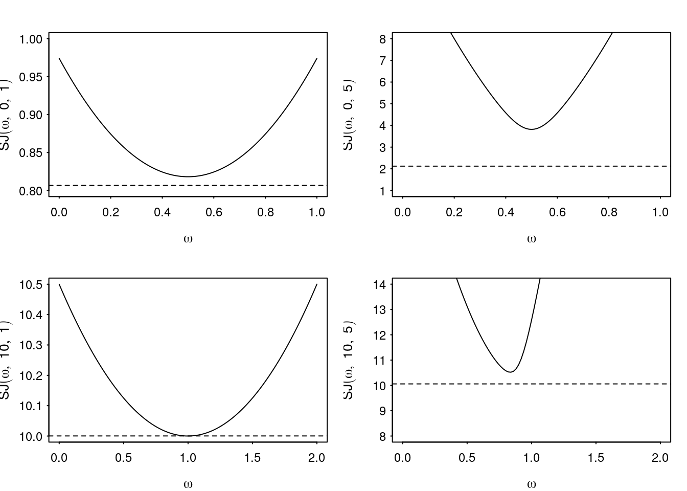
Figure 5: Examples of Saul-Jordan bound as a function of \(\omega\) for varying \(\mu\) and \(\sigma\).
If we apply the above bound to the relevant term in the ELBO we then have an new lower bound for the likelihood term \[ \begin{aligned} \mathbb E_q[\ln p(y|\beta)] &= \mathbb E_q[y^\top X\beta] - 1^\top\mathbb E_q[\ln(1 + \exp(X\beta))] \\ &\geq y^\top X\mu_\beta - \frac{1}{2}(\omega^2)^\top\text{diag}(X\Sigma_\beta X^\top) - \\ &\quad1^\top\ln\left[1+\exp(X\mu_\beta+\frac{1}{2}(1-2\omega)\odot\text{diag}(X\Sigma_\beta X^\top)\right] \end{aligned} \]
We find the derivatives \[ \begin{aligned} \mathsf{D}_{\omega} \mathcal{L}(q) &= \left[\text{expit}\left\{X\mu_\beta+\frac{1}{2}(1-2\omega)\odot\text{diag}\left(X\Sigma_\beta X^\top\right)\right\} - \omega\right]\odot\text{diag}(X\Sigma_\beta X^\top)\\ \mathsf{D}_{\mu_\beta} \mathcal{L}(q) &= X^\top\left[y- \text{expit}\left(X\mu_\beta+\frac{1}{2}(1-2\omega)\odot\text{diag}\left(X\Sigma_\beta X^\top\right)\right)\right]-\Sigma_0^{-1}(\mu_\beta-\mu_0)\\ \mathsf{H}_{\mu_\beta}\mathcal{L}(q) &= -X^\top\left(\frac{1}{2}\frac{1}{1+\cosh\left[X\mu_\beta+\frac{1}{2}(1-2\omega)\odot\text{diag}(X\Sigma_\beta X^\top)\right]}\right)X-\Sigma_0^{-1}. \end{aligned} \] Using the standard results in Rhode and Wand (2016) and setting \(\mathsf{D}_{\omega}\mathcal{L}(q)=0\) we find the updates \[ \begin{cases} \omega_0 &\leftarrow X\mu_\beta+\frac{1}{2}(1-2\omega)\odot\text{diag}(X\Sigma_\beta X^\top) \\ \omega_1 &\leftarrow \text{expit}(\omega_0) \\ \omega_2 &\leftarrow \frac{1}{2(1+\cosh(\omega_0))}\\ \nu_\beta &\leftarrow X^\top(y-\omega_1)-\Sigma_0^{-1}(\mu_\beta-\mu_0)\\ \Sigma_\beta &\leftarrow \left(X^\top\text{diag}(\omega_2)X+\Sigma_0^{-1}\right)^{-1}\\ \mu_\beta &\leftarrow \mu_\beta + \Sigma_\beta\nu_\beta \end{cases} \] and the lower bound \[ \begin{aligned} \mathcal{L}(q;\omega) &= \frac{d}{2} + \frac{1}{2}\ln|\Sigma_\beta| - \frac{1}{2}\ln|\Sigma_0| \\ &\quad -\frac{1}{2}\text{tr}(\Sigma^{-1}_0\Sigma)-\frac{1}{2}(\mu_\beta-\mu_0)\Sigma_0^{-1}(\mu_\beta-\mu_0) \\ &\quad +y^\top X\mu_\beta - \frac{1}{2}(\omega^2)^\top\text{diag}\left(X\Sigma_\beta X^\top\right) \\ &\quad -1^\top\ln\left(1 + \exp(X\mu_\beta + \frac{1}{2}(1-2\omega)\odot\text{diag}(X\Sigma_\beta X^\top))\right) \end{aligned} \]
Examples
The variational approximations were implemented in R.
b_psi <- function(psi) {
  psi/4 - plogis(psi)
}
c_psi <- function(psi) {
  psi^2/8 - psi*plogis(psi) + log(1 + exp(psi))
}

bb_log_reg <- function(
  X, y,
  mu0 = rep(0, ncol(X)), Sigma0 = diag(1, ncol(X)),
  maxiter = 100, tol = 1e-8, verbose = TRUE
) {

  d <- ncol(X)
  n <- nrow(X)
  invSigma0 <- solve(Sigma0)
  invSigma0_x_mu0 <- invSigma0 %*% mu0
  mu <- mu0
  Sigma <- Sigma0
  psi <- X %*% mu

  lb <- numeric(maxiter)
  i <- 0
  converged <- FALSE
  if(verbose) cat("\nStarting Bohning's bound optimisation:\n")
  while(i <= maxiter & !converged) {
    i <- i + 1
    psi <- X %*% mu
    Sigma <- solve(crossprod(X, X)/4 + invSigma0)
    mu <- (Sigma %*% (invSigma0_x_mu0 + crossprod(X, y + b_psi(psi))))[, 1]
    lb[i] <- 0.5*d + 0.5*log(det(Sigma)) - 0.5*log(det(Sigma0)) -
      0.5*crossprod(mu - mu0, invSigma0 %*% (mu - mu0)) - 0.5*sum(diag(invSigma0 %*% Sigma)) +
      crossprod(y, X %*% mu) -
      1/8*sum(diag(X %*% (Sigma + mu %o% mu) %*% t(X))) + crossprod(b_psi(psi), X %*% mu) - sum(c_psi(psi))

    if(verbose) cat(sprintf("Iteration %3d, ELBO = %5.10f\n", i, lb[i]))
    if(i > 1 && abs(lb[i] - lb[i - 1]) < tol) converged <- TRUE
  }
  return(list(lb = lb[1:i], mu = mu, Sigma = Sigma, psi = psi))
}

jj_log_reg <- function(
  X, y,
  mu0 = rep(0, ncol(X)), Sigma0 = diag(1, ncol(X)),
  maxiter = 100, tol = 1e-8, verbose = TRUE) {

  d <- ncol(X)
  n <- nrow(X)
  invSigma0 <- solve(Sigma0)
  invSigma0_x_mu0 <- invSigma0 %*% mu0
  mu <- mu0
  Sigma <- Sigma0
  xi <- y
  Xy <- crossprod(X, y - 0.5)

  lb <- numeric(maxiter)
  i <- 0
  converged <- FALSE
  if(verbose) cat("\nStarting Jaakkola-Jordan optimisation:\n")
  while(i <= maxiter & !converged) {
    i <- i + 1
    Xi <- Sigma + mu %o% mu
    xi <- sqrt(diag(X %*% Xi %*% t(X)))
    Sigma <- solve(crossprod(X, diag(tanh(xi/2)/(2*xi)) %*% X) + invSigma0)
    mu <- (Sigma %*% (Xy + invSigma0_x_mu0))[, 1]
    lb[i] <- 0.5*log(det(Sigma)) - 0.5*log(det(Sigma0)) +
      0.5*crossprod(mu, solve(Sigma) %*% mu) - 0.5*crossprod(mu0, invSigma0_x_mu0) +
      sum(0.5*xi - log(1 + exp(xi)) + (xi/4)*tanh(xi/2))


    if(verbose) cat(sprintf("Iteration %3d, ELBO = %5.10f\n", i, lb[i]))
    if(i > 1 && abs(lb[i] - lb[i - 1]) < tol) converged <- TRUE
  }
  return(list(lb = lb[1:i], mu = mu, Sigma = Sigma, xi = xi))
}

sj_log_reg <- function(
    X, y,
  mu0 = rep(0, ncol(X)), Sigma0 = diag(1, ncol(X)),
  maxiter = 100, tol = 1e-8, verbose = TRUE, muinit = mu0, Sigmainit = Sigma0) {

  d <- ncol(X)
  n <- nrow(X)
  invSigma0 <- solve(Sigma0)
  invSigma0_x_mu0 <- invSigma0 %*% mu0
  mu <- muinit
  Sigma <- Sigmainit
  omega1 <- y

  lb <- numeric(maxiter)
  i <- 0
  converged <- FALSE
  if(verbose) cat("\nStarting Saul-Jordan optimisation:\n")
  while(i <= maxiter & !converged) {
    i <- i + 1
    omega0 <- drop(X%*%mu + 0.5*(1 - 2*omega1) * diag(X%*%Sigma%*%t(X)))
    omega1 <- plogis(omega0)
    omega2 <- 1/(2*(1 + cosh(omega0)))
    nu <- crossprod(X, y - omega1) - invSigma0 %*% (mu - mu0)
    Sigma <- solve(crossprod(X, diag(omega2) %*% X) + invSigma0)
    mu <- (mu + Sigma %*% nu)

    lb[i] <- 0.5*d + 0.5*log(det(Sigma)) - 0.5*log(det(Sigma0)) -
      0.5*crossprod(mu - mu0, invSigma0 %*% (mu - mu0)) - 0.5*sum(diag(invSigma0 %*% Sigma)) +
      crossprod(y, X %*% mu) - 0.5*crossprod(omega1^2, diag(X %*% Sigma %*% t(X))) -
      sum(log(1 + exp(X %*% mu + 0.5 * (1 - 2*omega1) * diag(X %*% Sigma %*% t(X)))))

    if(verbose) cat(sprintf("Iteration %3d, ELBO = %5.10f\n", i, lb[i]))
    if(i > 1 && abs(lb[i] - lb[i - 1]) < tol) converged <- TRUE
  }
  return(list(lb = lb[1:i], mu = mu, Sigma = Sigma, omega1 = omega1))
}
// log_reg
data {
int<lower=0> N;
int<lower=1> P;
int<lower=0,upper=1> y[N];
matrix[N, P] X;
vector[P] mu0;
matrix[P, P] Sigma0;
}
parameters {
vector[P] beta;
}
model {
target += multi_normal_lpdf(beta | mu0, Sigma0);
target += bernoulli_logit_lpmf(y | X*beta);
}Below are a few examples of using the algorithms with approximations compared to posterior estimates obtained via Stan. We simulate data from a four parameter model under a weakly informative and strongly informative prior.
Example 1
library(rstan)
library(bridgesampling)

set.seed(123)
X <- cbind(1, runif(250), rnorm(250), sample(0:1, 250, replace = T))
y <- rbinom(250, 1, plogis(X %*% c(-4, 4, 0, 2)))

mc_fit <- sampling(log_reg, refresh = 0, iter = 1e4,
                   data = list(N = 250, P = 4, X = X, y = y, mu0 = rep(0,4), Sigma0 = diag(1,4)))
draws <- extract(mc_fit)$beta
ml_est <- bridge_sampler(mc_fit, silent = TRUE)
c("logm" = ml_est$logml, do.call(c, error_measures(ml_est)))
logm re2 cv
"-130.70016976142" "1.95159845904399e-07" "0.000441768996087773"
percentage
"0%" bb_fit <- bb_log_reg(X, y)
Starting Bohning's bound optimisation:
Iteration   1, ELBO = -136.6862931121
Iteration   2, ELBO = -132.1218471928
Iteration   3, ELBO = -131.5397621449
Iteration   4, ELBO = -131.4203424997
Iteration   5, ELBO = -131.3927353927
Iteration   6, ELBO = -131.3860285508
Iteration   7, ELBO = -131.3843613207
Iteration   8, ELBO = -131.3839422342
Iteration   9, ELBO = -131.3838363092
Iteration  10, ELBO = -131.3838094629
Iteration  11, ELBO = -131.3838026495
Iteration  12, ELBO = -131.3838009190
Iteration  13, ELBO = -131.3838004794
Iteration  14, ELBO = -131.3838003677
Iteration  15, ELBO = -131.3838003393
Iteration  16, ELBO = -131.3838003321
jj_fit <- jj_log_reg(X, y)
Starting Jaakkola-Jordan optimisation:
Iteration   1, ELBO = -138.1852835479
Iteration   2, ELBO = -131.2854654902
Iteration   3, ELBO = -131.1617743389
Iteration   4, ELBO = -131.1460168372
Iteration   5, ELBO = -131.1438972567
Iteration   6, ELBO = -131.1436093089
Iteration   7, ELBO = -131.1435700586
Iteration   8, ELBO = -131.1435647018
Iteration   9, ELBO = -131.1435639703
Iteration  10, ELBO = -131.1435638705
Iteration  11, ELBO = -131.1435638568
Iteration  12, ELBO = -131.1435638550
sj_fit <- sj_log_reg(X, y)
Starting Saul-Jordan optimisation:
Iteration   1, ELBO = -144.1383436591
Iteration   2, ELBO = -132.2772576553
Iteration   3, ELBO = -130.7474966363
Iteration   4, ELBO = -130.7203265204
Iteration   5, ELBO = -130.7197937190
Iteration   6, ELBO = -130.7197813211
Iteration   7, ELBO = -130.7197810128
Iteration   8, ELBO = -130.7197810047
Saul-Jordan bound is much tighter on the marginal likelihood compared to the other two bounds.
nice_par(mar = c(3,4,2,1))
x <- 1:max(length(bb_fit$lb), length(jj_fit$lb))
plot(bb_fit$lb, ylim = c(-132, -130), type = 'l', xlim = c(0,max(x)+4),
     xlab = expression(i), ylab = expression(ELBO(i)))
lines(1:length(jj_fit$lb), jj_fit$lb, lty = 1)
lines(1:length(sj_fit$lb), sj_fit$lb, lty = 1)
abline(h = ml_est$logml, lty = 2)
text(x = c(12, length(bb_fit$lb), length(jj_fit$lb), length(sj_fit$lb)),
     y = c(ml_est$logml+0.1, max(bb_fit$lb), max(jj_fit$lb), max(sj_fit$lb)),
     labels = c("MCMC Bridge Sampling", "Bohning", "Jaakkola-Jordan", "Saul-Jordan"),
     pos = 4, cex = 0.9)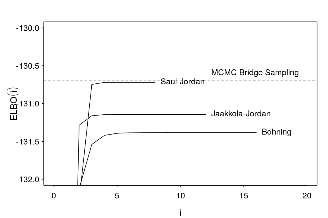
Figure 6: Comparison of evidence lower bounds with estimated marginal likelihood from bridge sampling of Stan posterior draws.
Tighter bound provides a better overall fit as evidenced by the comparisons in Figure 4.
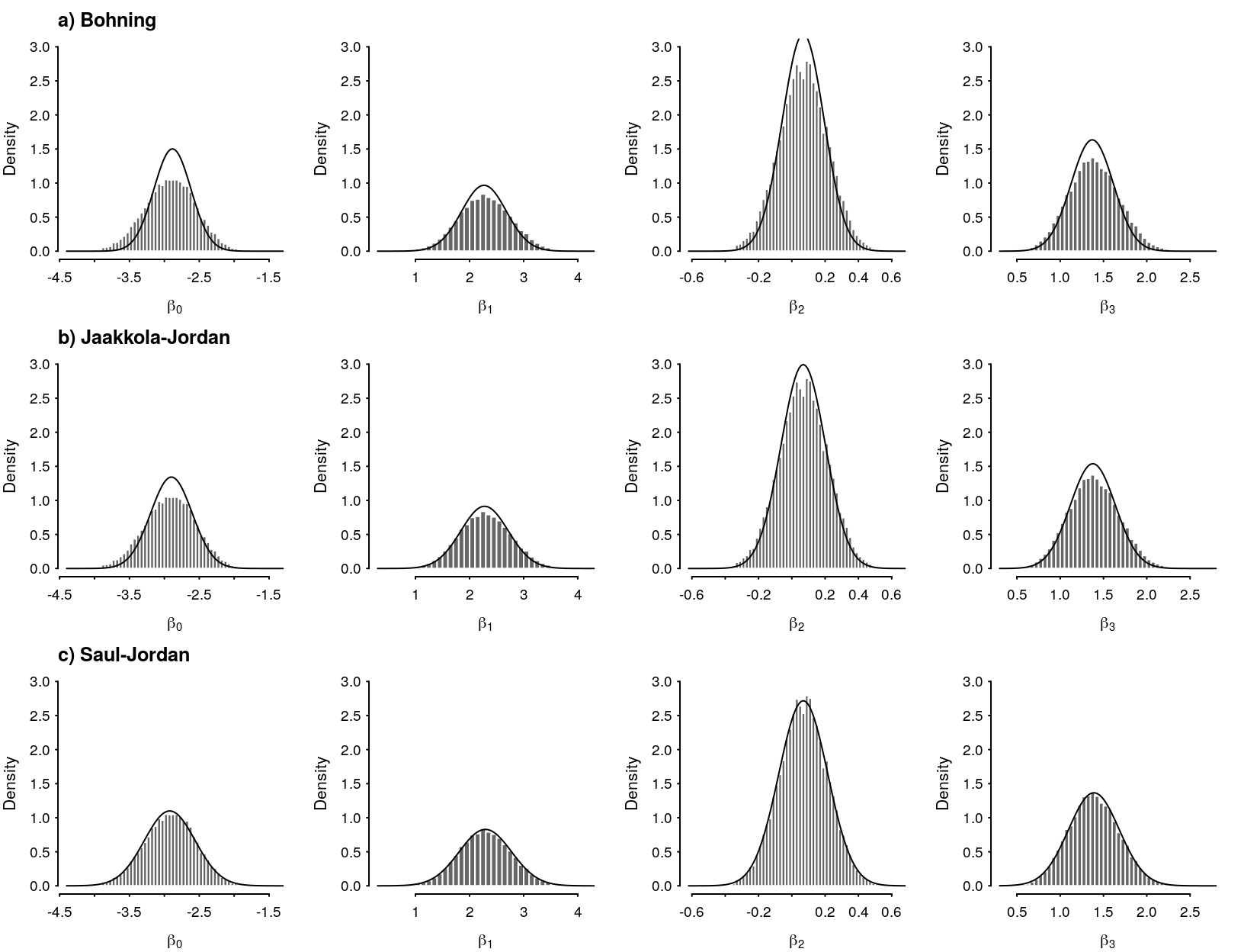
Figure 7: Comparison of MCMC and a) Bohning approximation, b) Jaakkola-Jordan approximation, c) Saul-Jordan approximation.
Example 2
Another example with a strongly informative prior.
set.seed(17)
n <- 50
X <- cbind(1, runif(n), rnorm(n), sample(0:1, n, replace = T))
y <- rbinom(n, 1, plogis(X %*% c(-4, 4, 0, 2)))
mu0 <- rep(5, 4)
Sigma0 <- diag(0.1, 4)

mc_fit <- sampling(log_reg, refresh = 0, iter = 1e4,
                   data = list(N = n, P = 4, X = X, y = y, mu0 = mu0, Sigma0 = Sigma0))
draws <- extract(mc_fit)$beta
ml_est <- bridge_sampler(mc_fit, silent = TRUE)
c("logm" = ml_est$logml, do.call(c, error_measures(ml_est)))
logm re2 cv
"-222.974712426576" "5.4166359728906e-08" "0.000232736674653794"
percentage
"0%" bb_fit <- bb_log_reg(X, y, mu0, Sigma0)
Starting Bohning's bound optimisation:
Iteration   1, ELBO = -253.3819353254
Iteration   2, ELBO = -235.9904529936
Iteration   3, ELBO = -228.8813246036
Iteration   4, ELBO = -225.9754733461
Iteration   5, ELBO = -224.7945801547
Iteration   6, ELBO = -224.3161162161
Iteration   7, ELBO = -224.1222873212
Iteration   8, ELBO = -224.0436426944
Iteration   9, ELBO = -224.0116608435
Iteration  10, ELBO = -223.9986249109
Iteration  11, ELBO = -223.9933005415
Iteration  12, ELBO = -223.9911222252
Iteration  13, ELBO = -223.9902298612
Iteration  14, ELBO = -223.9898639338
Iteration  15, ELBO = -223.9897137685
Iteration  16, ELBO = -223.9896521118
Iteration  17, ELBO = -223.9896267859
Iteration  18, ELBO = -223.9896163801
Iteration  19, ELBO = -223.9896121038
Iteration  20, ELBO = -223.9896103461
Iteration  21, ELBO = -223.9896096236
Iteration  22, ELBO = -223.9896093266
Iteration  23, ELBO = -223.9896092045
Iteration  24, ELBO = -223.9896091543
Iteration  25, ELBO = -223.9896091336
Iteration  26, ELBO = -223.9896091251
jj_fit <- jj_log_reg(X, y, mu0, Sigma0)
Starting Jaakkola-Jordan optimisation:
Iteration   1, ELBO = -234.1256982263
Iteration   2, ELBO = -224.0077883131
Iteration   3, ELBO = -223.3756601279
Iteration   4, ELBO = -223.3236753050
Iteration   5, ELBO = -223.3191115840
Iteration   6, ELBO = -223.3187028904
Iteration   7, ELBO = -223.3186660325
Iteration   8, ELBO = -223.3186626992
Iteration   9, ELBO = -223.3186623974
Iteration  10, ELBO = -223.3186623700
Iteration  11, ELBO = -223.3186623675
sj_fit <- sj_log_reg(X, y, mu0, Sigma0)
Starting Saul-Jordan optimisation:
Iteration   1, ELBO = -223.2681695675
Iteration   2, ELBO = -222.9814171756
Iteration   3, ELBO = -222.9777292984
Iteration   4, ELBO = -222.9776740965
Iteration   5, ELBO = -222.9776732546
Iteration   6, ELBO = -222.9776732418
Iteration   7, ELBO = -222.9776732416
nice_par(mar = c(3,4,2,1))
x <- 1:max(length(bb_fit$lb), length(jj_fit$lb))
plot(bb_fit$lb, type = 'l', ylim = c(-225, -222), xlim = c(0,max(x)+4),
xlab = expression(i), ylab = expression(ELBO(i)))
lines(1:length(jj_fit$lb), jj_fit$lb, lty = 1)
lines(1:length(sj_fit$lb), sj_fit$lb, lty = 1)
abline(h = ml_est$logml, lty = 2)
text(x = c(15, length(bb_fit$lb), length(jj_fit$lb), length(sj_fit$lb)),
y = c(ml_est$logml+0.1, max(bb_fit$lb), max(jj_fit$lb), max(sj_fit$lb)),
labels = c("MCMC Bridge Sampling", "Bohning", "Jaakkola-Jordan", "Saul-Jordan"),
pos = 4, cex = 0.9)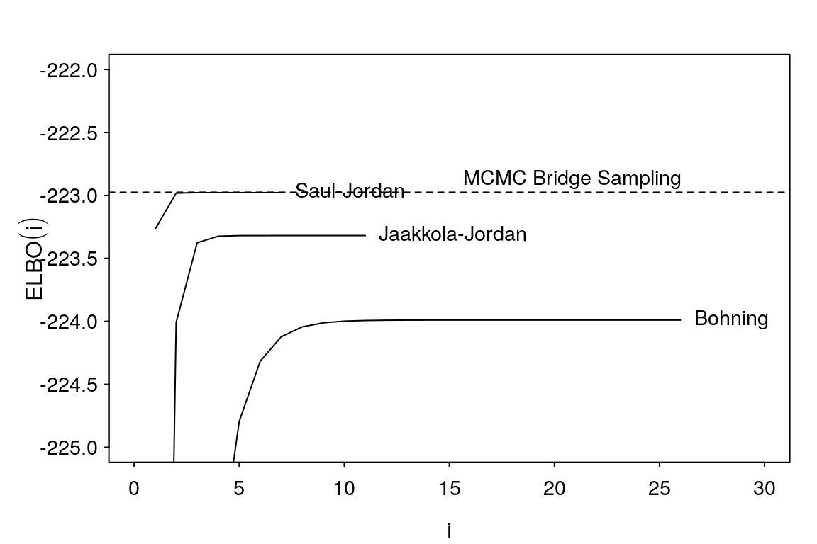
Figure 8: Comparison of evidence lower bounds with estimated marginal likelihood from bridge sampling of Stan posterior draws.
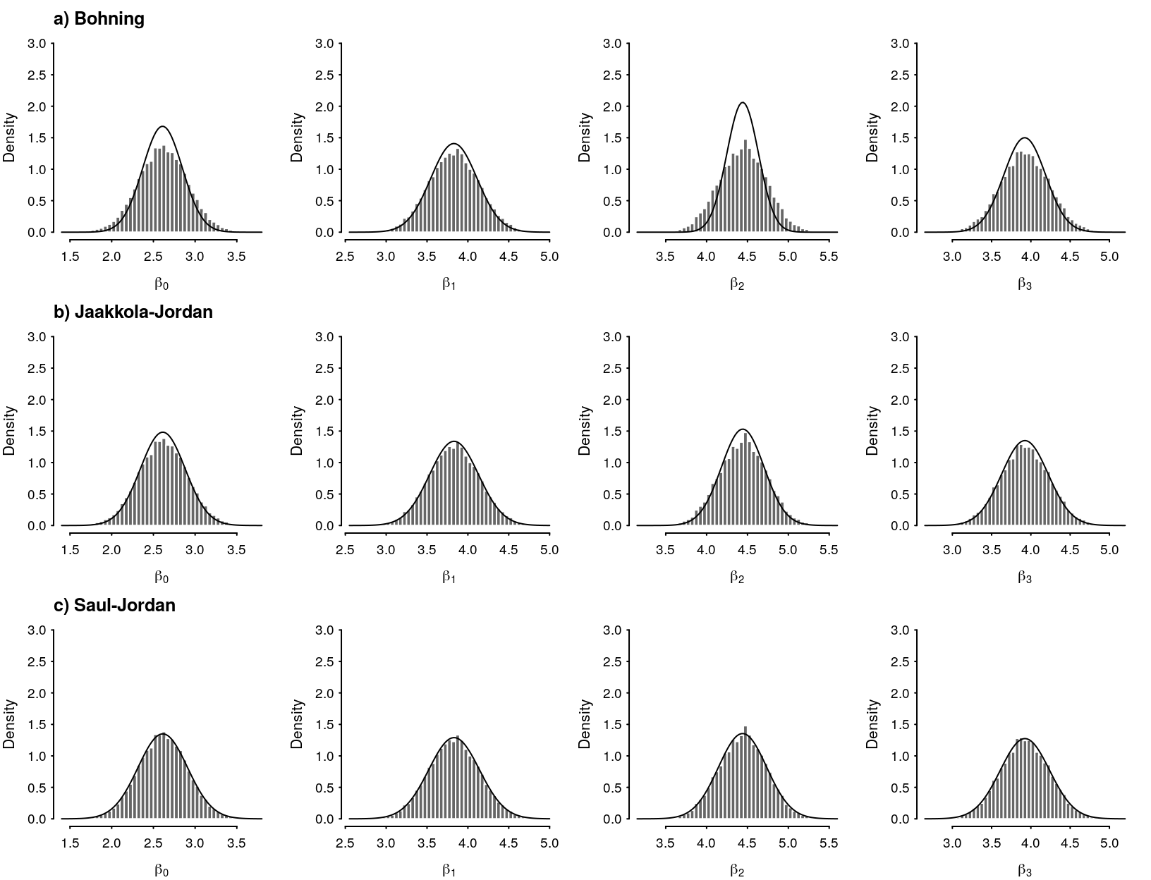
Figure 9: Comparison of MCMC and a) Bohning approximation, b) Jaakkola-Jordan approximation, c) Saul-Jordan approximation.
Example 3 (divergence)
In this instance we specify a diffuse prior \(\beta\sim N(0, 10I)\). In this case the Saul-Jordan updates diverge. This can be addressed by initalising with Jaakkola Jordan updates, and then switching to Saul-Jordan.
set.seed(17)
n <- 50
X <- cbind(1, runif(n), rnorm(n), sample(0:1, n, replace = T))
y <- rbinom(n, 1, plogis(X %*% c(-4, 4, 0, 2)))
mu0 <- rep(5, 4)
Sigma0 <- diag(10, 4)

mc_fit <- sampling(log_reg, refresh = 0, iter = 1e4,
                   data = list(N = n, P = 4, X = X, y = y, mu0 = mu0, Sigma0 = Sigma0))
draws <- extract(mc_fit)$beta
ml_est <- bridge_sampler(mc_fit, silent = TRUE)
c("logm" = ml_est$logml, do.call(c, error_measures(ml_est)))
logm re2 cv
"-37.4755263328553" "9.31771281055153e-07" "0.000965283005680279"
percentage
"0%" bb_fit <- bb_log_reg(X, y, mu0, Sigma0, tol= 1e-5)
Starting Bohning's bound optimisation:
Iteration   1, ELBO = -245.3022653704
Iteration   2, ELBO = -191.7385416887
Iteration   3, ELBO = -149.1998030217
Iteration   4, ELBO = -116.7759865866
Iteration   5, ELBO = -92.7062164260
Iteration   6, ELBO = -74.2998095254
Iteration   7, ELBO = -60.2835201941
Iteration   8, ELBO = -50.2994349160
Iteration   9, ELBO = -43.9822677319
Iteration  10, ELBO = -40.6595084573
Iteration  11, ELBO = -39.2383473863
Iteration  12, ELBO = -38.6794253982
Iteration  13, ELBO = -38.4572975512
Iteration  14, ELBO = -38.3725772737
Iteration  15, ELBO = -38.3425363564
Iteration  16, ELBO = -38.3325176974
Iteration  17, ELBO = -38.3293114406
Iteration  18, ELBO = -38.3283110015
Iteration  19, ELBO = -38.3280034372
Iteration  20, ELBO = -38.3279096809
Iteration  21, ELBO = -38.3278812366
Iteration  22, ELBO = -38.3278726298
jj_fit <- jj_log_reg(X, y, mu0, Sigma0, tol= 1e-5)
Starting Jaakkola-Jordan optimisation:
Iteration   1, ELBO = -137.1696439625
Iteration   2, ELBO = -43.8110602922
Iteration   3, ELBO = -38.9935822151
Iteration   4, ELBO = -38.1997101065
Iteration   5, ELBO = -38.0540172672
Iteration   6, ELBO = -38.0274586404
Iteration   7, ELBO = -38.0227440650
Iteration   8, ELBO = -38.0219208719
Iteration   9, ELBO = -38.0217782699
Iteration  10, ELBO = -38.0217536531
Iteration  11, ELBO = -38.0217494099
sj_fit <- sj_log_reg(X, y, mu0, Sigma0, tol= 1e-5, maxiter = 10)
Starting Saul-Jordan optimisation:
Iteration   1, ELBO = -532.6092716102
Iteration   2, ELBO = -3074.0150499361
Iteration   3, ELBO = -9060.7195618299
Iteration   4, ELBO =  -Inf
Iteration   5, ELBO = -11882.7451399044
Iteration   6, ELBO = -9286.6484948503
Iteration   7, ELBO = -12440.1807404176
Iteration   8, ELBO = -11138.4037374864
Iteration   9, ELBO = -14789.8026254242
Iteration  10, ELBO = -13518.9146389380
Iteration  11, ELBO = -16597.9913846932
jj_sj_fit <- sj_log_reg(X, y, mu0, Sigma0, tol= 1e-5, maxiter = 10, muinit = jj_fit$mu, Sigmainit = jj_fit$Sigma)
Starting Saul-Jordan optimisation:
Iteration   1, ELBO = -37.5931435978
Iteration   2, ELBO = -37.5790440387
Iteration   3, ELBO = -37.5780978548
Iteration   4, ELBO = -37.5779489790
Iteration   5, ELBO = -37.5779192108
Iteration   6, ELBO = -37.5779124936
Summary
Bohning’s bound provides the weakest approximation of the three methods considered here. Evidence seems to suggest that the Jaakkola-Jordan updates are a more stable approximation but less accurate, whereas Saul-Jordan provides a tighter bound but may diverge in instances of high correlation between the posterior parameters or diffuse priors. A usual recommendation is to initialise with Jaakkola-Jordan updates until convergence or some number of iterations are completed, and then switch to using Saul-Jordan updates to improve the bound.
In a future post I aim to look at the use of quadrature rules to calculate the expectation directly rather using approximation bounds.
Useful Identities
\[ \begin{aligned} \text{expit}(x) &= \frac{1}{2} + \frac{\tanh(x/2)}{2} \\ \frac{d}{dx} \ln\left(1+e^{f(x)}\right) &= f^\prime(x)\text{expit}\left(f(x)\right)\\ \frac{d}{dx} \text{expit}\left(f(x)\right) &= \frac{f^\prime(x)}{2\left(1 + \cosh\left(f(x)\right)\right)}\\ x^\top A x=\text{tr}(x^\top A x) = \text{tr}(Axx^\top)&\implies\mathbb E[x^\top A x] = \text{tr}\left(\mathbb E[xx^\top]A\right)=\text{tr}(A\mathbb V[x])+\mathbb E[x]^\top A\mathbb E[x] \end{aligned} \]
References
Böhning, Dankmar. 1992. “Multinomial Logistic Regression Algorithm.” Annals of the Institute of Statistical Mathematics 44 (1): 197–200.
Böhning, Dankmar, and Bruce G Lindsay. 1988. “Monotonicity of Quadratic-Approximation Algorithms.” Annals of the Institute of Statistical Mathematics 40 (4): 641–63.
Durante, Daniele, and Tommaso Rigon. 2017. “Conditionally Conjugate Mean-Field Variational Bayes for Logistic Models.” arXiv Preprint arXiv:1711.06999.
Jaakkola, Tommi S, and Michael I Jordan. 2000. “Bayesian Parameter Estimation via Variational Methods.” Statistics and Computing 10 (1): 25–37.
Murphy, Kevin P. 2012. Machine Learning: A Probabilistic Perspective. MIT press.
Nolan, Tui H, and Matt P Wand. 2017. “Accurate Logistic Variational Message Passing: Algebraic and Numerical Details.” Stat 6 (1): 102–12.
Polson, Nicholas G, James G Scott, and Jesse Windle. 2013. “Bayesian Inference for Logistic Models Using Pólya–Gamma Latent Variables.” Journal of the American Statistical Association 108 (504): 1339–49.
Rhode, David, and Matt P. Wand. 2016. “Semiparametric Mean Field Variational Bayes: General Principles and Numerical Issues.” Journal of Machine Learning Research 17: 1–47.
Wand, Matt P. 2017. “Fast Approximate Inference for Arbitrarily Large Semiparametric Regression Models via Message Passing.” Journal of the American Statistical Association 112 (517): 137–68.