Background
I was recently tasked with providing support to a study where the primary outcome was an eight-item, seven-point Likert scale. The proposal was to use a t-test to undertake the analysis. Being unfamiliar with the analysis of Likert scale responses I decided to do a bit of research into what was standard practice.
There appears to be disagreement about whether the appropriate analysis should be based on parametric or non-parametric methods (Sullivan and Artino Jr 2013). Technically, Likert scale data are ordinal, and any values assigned to the levels beyond the natural ordering are arbitrary. However, there still appears to be various recommendations on the appropriateness of parametric methods which ignore this ordinal nature and impose interval values to each Likert items possible responses (Carifio and Perla 2008; Norman 2010; Harpe 2015).
Despite these recommendations, I feel somewhat unsatisfied using models which fail to represent a reasonable data generating process. Some arguments to this end are made in Liddell and Kruschke (2018), where the suggestion is, unsurprisingly, to use ordinal models to analyse ordinal data. The authors present a number of scenarios where assuming an ordinal model can better capture certain potential patterns of Likert scale data.
Further details on estimating Bayesian ordinal models in R using brms are given by the package author in Bürkner and Vuorre (2018).
I wanted to work through the application of ordinal models to Likert scale data, including simulation, sample size calculation, and where the benefits and, if any, disadvantages may come into play.
Likert Scale Data
Likert (pron: LICK-ert) data are ordered responses or ratings to questions commonly collected via surveys. Response options are usually symmetrical (e.g. disagree, somewhat disagree, somewhat agree, agree, etc.) and contain an indifferent midpoint response (e.g. neutral, neither agree nor disagree).
Technically, a Likert item is a single question, and a Likert scale is a collection of Likert items viewed together as a collective measure of some trait of interest. I find this to be a key point in the appeal of a latent variable interpretation to Likert scale data. We are interested in some underlying trait which cannot be measured directly, so instead we use a tool of survey questions which all aim to measure in varying degrees this trait of interest. This implies that an individuals responses to Likert items should be correlated within the scale, as they all aim to measure the same underlying trait. This notion and some of its advantages are also outlined in Fox (2010).
Despite the intuitive notion of a latent trait of interest, what appears to be the most common approach to analysing Likert scale data is to model the responses directly by mapping them to an interval scale. For example: strongly disagree = 1, disagree = 2, neutral = 3, agree = 4, strongly agree = 5. This mapping maintains the ordering but introduces an assumed metric on responses, e.g. the distance between strongly disagree and disagree is equal to the distance between disagree and neutral. For each item on a \(K\)-point response scale, only \(K\) values are possible, and on a Likert scale comprised of \(Q\) items where analysis is based on the item averaged responses for each individual, the only possible values for an individuals item-averaged responses are \[ \bar Y \in \{1,(Q+1)/Q,(Q+2)/Q,...,(QK-1)/Q,K\}. \]
This metric is arbitrary, we may well equally justify that strongly disagree is further from disagree than disagree is from neutral and similarly for agree and strongly agree. This could be represented by adjusting the mapping, e.g. strongly disagree = 1, disagree = 3, neutral = 4, agree = 5, and strongly agree = 7, say. In the case of multiple Likert items forming the scale, the veraged score is analysed according to the continuous metric by a t-test or linear regression.
A common alternative is to avoid parametric assumptions and instead rely on rank tests, such as Mann-Whitney U and Kruskal-Wallis. These may be reasonable for a single Likert item, however, when combining Likert items into a scale it’s unclear to me why analysing aggregated ranks should be the approach, rather than analysing item specific ranks and incorporating these results across items.
The key problem I have with the above approaches is that neither provides a model for the data generating process. There is no coherent mechanism implied which could be used to simulate Likert scale data. Sure, we could assume some discrete distribution over the responses within each item, simulate data, and conduct an analysis, but the simulated data in no way relates to the model assumed for analysis.
A reasonable model for the Likert scale should be able to generate data which is consistent with what could actually be observed in reality.
Ordinal Models for Likert Scale Data
Although not intuitive for all ordinal data, the concept of a continuous latent variable underlying the ordinal responses to Likert scale data is appealing.
For an individual \(i\), we are interested in the underlying unobservable trait \(Y_i^\star\in\mathbb R\) as measured by their Likert scale responses.
We observe some random vector \(Y_i=(Y_{i1},...,Y_{iQ})\) giving an individuals responses to all of the \(Q\) items, with the response to item \(q\in\{1,...,Q\}\) being made on a \(K_q\)-point scale, that is \(Y_{iq}\in\{1,...,K_q\}\). Generally, \(K_q=K\) for all \(q\in\{1,...,Q\}\). We assume the individuals responses for an item \(q\) is governed by a continuous latent trait vector, \(Y_i^\star = (Y_{i1}^\star,...,Y_{iQ}^\star)\in\mathbb R^Q\) according to \(K_q-1\) thresholds, \(-\infty=\tau_{q,0}<\tau_{q,1}<\cdots<\tau_{q,K_q-1}<\tau_{q,K_q}=\infty\),
The value of \(Y_i^\star\) then determines the responses \(Y_i\) by \[ Y_{iq} = k \iff Y_{iq}^\star \in (\tau_{q,k-1},\tau_{q,k}],\quad q\in\{1,...,Q\} \]
We have assumed that each Likert item relates to its own latent trait, however, for Likert scale data, all items by construction are meant to measure the same trait of interest, and therefore, we might prefer to assume a singular latent variable which governs all responses. Additionally, we might assume that thresholds are constant across items, that is \(\tau_{q,k} = \tau_k\) for all \(q\).
To model the latent trait, we may assume \[ Y_{iq}^\star = \mu_{iq} + \sigma_{iq}\epsilon_{iq} \] where \(\epsilon\sim F(\cdot)\) for some location-scale family distribution \(F\). Usual choices are normal, logistic, and Gumbel (extreme value) distributions.
Then, \[ \begin{aligned} \mathbb P(Y_{iq} \leq k|\mu_{iq},\sigma_{iq}) &= \mathbb P(Y_{iq}^\star\leq\tau_{q,k}|\mu_{iq},\sigma_{iq}) \\ &= \mathbb P(\mu_{iq} + \sigma_{iq}\epsilon_{iq}\leq\tau_{q,k}|\mu_{iq},\sigma_{iq}) \\ &= \mathbb P\left(\epsilon_{iq} \leq \frac{\tau_{q,k} - \mu_{iq}}{\sigma_{iq}}|\mu_{iq},\sigma_{iq}\right) \\ &= F\left(\frac{\tau_{q,k} - \mu_{iq}}{\sigma_{iq}}|\mu_{iq},\sigma_{iq}\right). \end{aligned} \] From this, the discrete probability function for each response item can be calculated \[ \begin{aligned} \mathbb P(Y_{iq} = k) &= \mathbb P(Y_{iq} \leq k) - \mathbb P(Y_{iq} < k) \\ &= F\left(\frac{\tau_{q,k} - \mu_{iq}}{\sigma_{iq}}|\mu_{iq},\sigma_{iq}\right) - F\left(\frac{\tau_{q,k-1} - \mu_{iq}}{\sigma_{iq}}|\mu_{iq},\sigma_{iq}\right). \end{aligned} \] We could equivalently define probababilities in the other direction Then, \[ \begin{aligned} \mathbb P(Y_{iq} > k|\mu_{iq},\sigma_{iq}) &= \mathbb P(Y_{iq}^\star>\tau_{qk}|\mu_{iq},\sigma_{iq}) \\ &= \mathbb P(\mu_{iq} + \sigma_{iq}\epsilon_{iq}>\tau_{qk}|\mu_{iq},\sigma_{iq}) \\ &= \mathbb P\left(\epsilon_{iq} > \frac{\tau_{qk} - \mu_{iq}}{\sigma_{iq}}|\mu_{iq},\sigma_{iq}\right) \\ &= F\left(\frac{\mu_{iq} - \tau_{qk}}{\sigma_{iq}}|\mu_{iq},\sigma_{iq}\right). \end{aligned} \]
Individual-level and item-level effects can then be incoroporated via \(\mu_{iq}\) and \(\sigma_{iq}\). A simple approach is to assume a constant baseline mean and variance which are adjusted by additional covariates \[ \begin{aligned} Y_{iq}^\star &= \mu_{iq} + \sigma_{iq}\epsilon_{iq} \\ &= \mu_0 + X_i\beta + \sigma\epsilon_i. \end{aligned} \]
One issue when it comes to estimation is that the model is overparameterised: a change in the threshold value can be compensated for by a change in the linear predictor value. E.g. if \(\tau_{q,k}^\star = \tau_{q,k} + c\) then take \(\mu_{iq}^\star = \mu_{iq} + c\). Similarly, a change in the variance can be compensated for by a rescaling of the thresholds and mean. The common approach is to fix the location and scale parameters and/or as many threshold parameters as necessary to make the model identifiable. Usually it may be enough to:
- fix the location and scale parameters \(\mu_0 = 0\) and \(\sigma=1\).
- fix the boundary threshold parameters \(\tau_{q,1}\) and \(\tau_{q,K_q-1}\).
Liddell and Kruschke (2018) propose an intuitive parameterisation where \(\tau_1=1.5\) and \(\tau_{K-1}=K-0.5\) are fixed. In this way, the base mean \(\mu_0\) is interpreted intuitively as the value of the averaged items.
Examples
library(rstan)
library(brms)
library(bayesplot)
library(dplyr)
library(tidyr)
library(mvtnorm)
library(ordinal)
Parametric
One-item example
Suppose that for each of \(n\) individuals, \(Y_i^\star \sim D(\mu_i,\sigma)\) for \(D\in\{N, L, G\}\) with the value of \(Y_i\) governed by thresholds \(\tau_{1:4} = (-1,-0.5,0.5,1)\).
We assume a reasonably large sample size of \(n=500\) to recover the true parameter values within reasonable variation.
dgumbel <- function(x, mu = 0, sigma = 1, log = FALSE) {
  z <- (x - mu) / sigma
  l <- -log(sigma) - (z + exp(-z))
  if(log)
    return(l)
  else
    return(exp(l))
}
pgumbel <- function(x, mu = 0, sigma = 1, log = FALSE) {
  z <- (x - mu) / sigma
  l <- -exp(-z)
  if(log)
    exp(l)
  else
    return(exp(l))
}
rgumbel <- function(n, mu = 0, sigma = 1) {
  mu - sigma * log( - log(runif(n)))
}
tau <- c(-1.5, -1, -0.5, 0.5, 1, 1.5)
K <- length(tau) + 1
p1 <- diff(c(0, pnorm(tau), 1))
p2 <- diff(c(0, plogis(tau), 1))
p3 <- diff(c(0, pgumbel(tau), 1))
par(mfrow = c(2,2), mar = c(4,4.5,2,1), oma = c(0,0,0,0))
curve(dnorm(x), xlim = c(-10, 10), xlab = expression(y^{"*"}), ylab = expression(f(y^{"*"})), main = "a) Latent")
curve(dlogis(x), add = T, lty = 2)
curve(dgumbel(x), add = T, lty = 3)
legend("topleft", legend = c("Normal", "Logistic", "Gumbel"), lty = 1:3, bty = 'n')
plot(1:K, p1, type = 'h', ylim = c(0, 0.5), ylab = expression(f(y)), xlab = "y", main = "b) Normal")
plot(1:K, p2, type = 'h', ylim = c(0, 0.5), ylab = expression(f(y)), xlab = "y", main = "c) Logistic")
plot(1:K, p3, type = 'h', ylim = c(0, 0.5), ylab = expression(f(y)), xlab = "y", main = "d) Gumbel")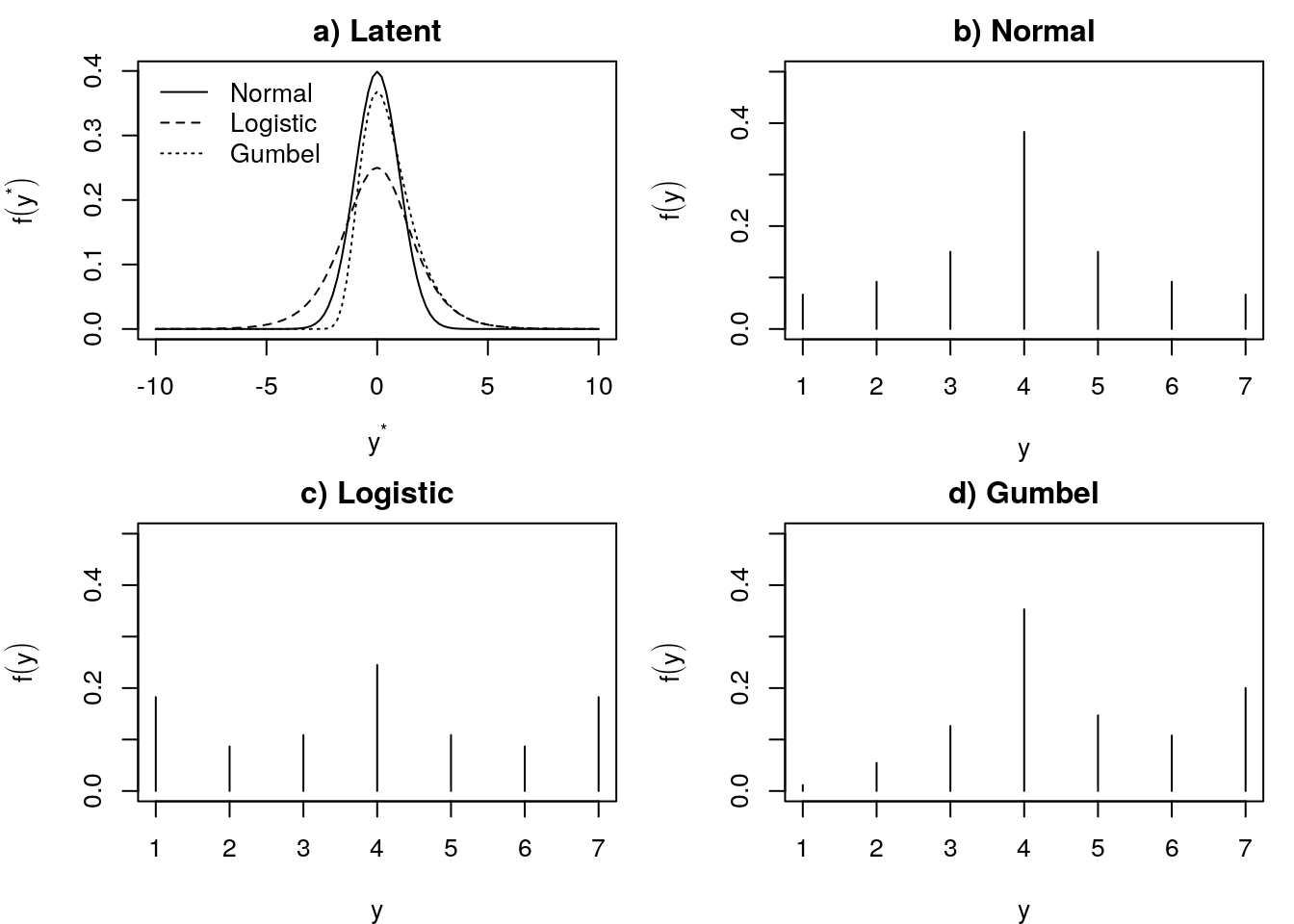
Figure 1: Latent variable and response variable for normal, logistic, and Gumbel distributions with thresholds \(\tau=(-1.5,-1.0,-0.5,0.5,1.0,1.5)\).
gen_one_item_data <- function(n, mu = 0, sig = 1, tau = c(-1, -0.5, 0.5, 1), dist = "normal") {
  rgen <- switch(dist,
    normal = rnorm,
    logistic = rlogis,
    gumbel = rgumbel
  )
  y_star <- rgen(n, mu, sig)
  y <- findInterval(y_star, c(-Inf, tau, Inf))
  return(y)
}
// one_item_model
data {
int<lower=1> N;
int<lower=1> P;
int<lower=1> K;
int<lower=1,upper=K> y[N];
row_vector[P] x[N];
}
parameters {
vector[P] beta;
ordered[K-1] tau;
}
model {
vector[K] p;
beta ~ normal(0, 10);
for(n in 1:N) {
real eta;
eta = x[n]*beta;
p[1] = Phi(tau[1] - eta);
for(k in 2:(K-1))
p[k] = Phi(tau[k] - eta) - Phi(tau[k-1] - eta);
p[K] = 1 - Phi(tau[K-1] - eta);
y[n] ~ categorical(p);
}
}// one_item_model_alt
data {
int<lower=1> N;
int<lower=1> P;
int<lower=1> K;
int<lower=1,upper=K> y[N];
row_vector[P] x[N];
}
parameters {
real<lower=0> sigma;
vector[P] beta;
ordered[K-3] tau;
}
transformed parameters {
ordered[K-1] tau_all;
tau_all[1] = 1.5;
tau_all[K-1] = K - 0.5;
tau_all[2:(K-2)] = tau;
}
model {
vector[K] p;
beta ~ normal(0, 10);
for(n in 1:N) {
real eta;
eta = x[n]*beta;
p[1] = Phi((tau_all[1] - eta) / sigma);
for(k in 2:(K-1))
p[k] = Phi((tau_all[k] - eta) / sigma) - Phi((tau_all[k-1] - eta) / sigma);
p[K] = 1 - Phi((tau_all[K-1] - eta) / sigma);
y[n] ~ categorical(p);
}
}N <- 500
b <- 1
tau <- c(-1.5, -0.5, 0.5, 1.5)
K <- length(tau) + 1
x <- rep(c(0, 1), each = N / 2)
m <- x*b
y <- gen_one_item_data(N, m, 1)
# ystar <- rnorm(N, m, 1)
# y <- findInterval(ystar, c(-Inf, tau, Inf))
p1 <- diff(c(0, pnorm(tau), 1))
p2 <- diff(c(0, pnorm(tau - 1), 1))
cbind("Pop value (x = 0)" = p1, "Pop value (x = 1)" = p2, prop.table(table(y, x), 2))## Pop value (x = 0) Pop value (x = 1) 0 1
## 1 0.0668072 0.006209665 0.164 0.024
## 2 0.2417303 0.060597536 0.116 0.044
## 3 0.3829249 0.241730337 0.400 0.196
## 4 0.2417303 0.382924923 0.160 0.192
## 5 0.0668072 0.308537539 0.160 0.544c("Population value" = sum(p1*1:K), "Sample value" = mean(y[x == 0]))## Population value Sample value
## 3.000 3.036c("Population value" = sum(p2*1:K), "Sample value" = mean(y[x == 1]))## Population value Sample value
## 3.926983 4.188000dat <- list(N = N, K = 5, P = 1, y = y, x = cbind(x))
fit <- sampling(one_item_model, data = dat, refresh = 0)
dat <- list(N = N, K = 5, P = 2, y = y, x = cbind(1, x))
fit_alt <- sampling(one_item_model_alt, data = dat, refresh = 0)## Warning: The largest R-hat is NA, indicating chains have not mixed.
## Running the chains for more iterations may help. See
## http://mc-stan.org/misc/warnings.html#r-hat## Warning: Bulk Effective Samples Size (ESS) is too low, indicating posterior means and medians may be unreliable.
## Running the chains for more iterations may help. See
## http://mc-stan.org/misc/warnings.html#bulk-ess## Warning: Tail Effective Samples Size (ESS) is too low, indicating posterior variances and tail quantiles may be unreliable.
## Running the chains for more iterations may help. See
## http://mc-stan.org/misc/warnings.html#tail-essprint(fit)## Inference for Stan model: 30a6fb43fd8f0f817443ccb0218ae9f6.
## 4 chains, each with iter=2000; warmup=1000; thin=1;
## post-warmup draws per chain=1000, total post-warmup draws=4000.
##
## mean se_mean sd 2.5% 25% 50% 75% 97.5% n_eff Rhat
## beta[1] 1.06 0.00 0.10 0.86 0.99 1.06 1.13 1.25 3701 1
## tau[1] -0.97 0.00 0.09 -1.15 -1.03 -0.97 -0.91 -0.79 2986 1
## tau[2] -0.54 0.00 0.08 -0.69 -0.60 -0.54 -0.49 -0.39 3716 1
## tau[3] 0.44 0.00 0.08 0.30 0.39 0.44 0.49 0.59 3739 1
## tau[4] 0.97 0.00 0.08 0.81 0.91 0.97 1.02 1.13 3568 1
## lp__ -678.36 0.04 1.59 -682.42 -679.10 -678.03 -677.21 -676.34 1656 1
##
## Samples were drawn using NUTS(diag_e) at Thu Apr 30 15:49:51 2020.
## For each parameter, n_eff is a crude measure of effective sample size,
## and Rhat is the potential scale reduction factor on split chains (at
## convergence, Rhat=1).print(fit_alt)## Inference for Stan model: 1c4e6e118a80c225f30d92859ecb91cd.
## 4 chains, each with iter=2000; warmup=1000; thin=1;
## post-warmup draws per chain=1000, total post-warmup draws=4000.
##
## mean se_mean sd 2.5% 25% 50% 75% 97.5% n_eff
## sigma 1.58 0.00 0.08 1.42 1.52 1.57 1.63 1.74 3380
## beta[1] 3.00 0.00 0.11 2.77 2.92 3.00 3.07 3.21 2476
## beta[2] 1.65 0.00 0.16 1.34 1.54 1.65 1.76 1.98 2364
## tau[1] 2.15 0.00 0.08 1.99 2.09 2.15 2.20 2.32 2663
## tau[2] 3.68 0.00 0.07 3.54 3.63 3.68 3.73 3.82 4263
## tau_all[1] 1.50 NaN 0.00 1.50 1.50 1.50 1.50 1.50 NaN
## tau_all[2] 2.15 0.00 0.08 1.99 2.09 2.15 2.20 2.32 2663
## tau_all[3] 3.68 0.00 0.07 3.54 3.63 3.68 3.73 3.82 4263
## tau_all[4] 4.50 NaN 0.00 4.50 4.50 4.50 4.50 4.50 NaN
## lp__ -676.14 0.04 1.57 -679.94 -676.96 -675.86 -675.00 -674.04 1576
## Rhat
## sigma 1
## beta[1] 1
## beta[2] 1
## tau[1] 1
## tau[2] 1
## tau_all[1] NaN
## tau_all[2] 1
## tau_all[3] 1
## tau_all[4] NaN
## lp__ 1
##
## Samples were drawn using NUTS(diag_e) at Thu Apr 30 15:50:11 2020.
## For each parameter, n_eff is a crude measure of effective sample size,
## and Rhat is the potential scale reduction factor on split chains (at
## convergence, Rhat=1).plot(fit, plotfun = "hist", bins = 50)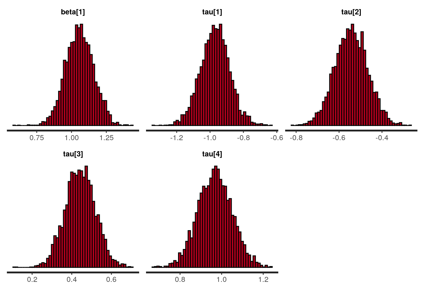
plot(fit_alt, par = c("sigma", "beta", "tau[1]", "tau[2]"), plotfun = "hist", bins = 50)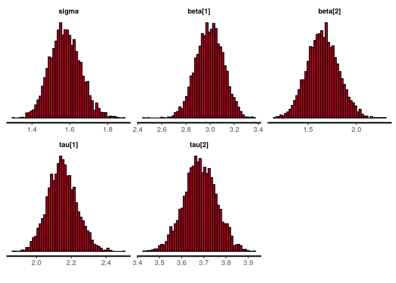
s1 <- as.matrix(fit)
s2 <- as.matrix(fit_alt)

tau2 <- s1[, 3]
tau2alt <- (s2[, 7] - s2[, 2]) / s2[, 1]
cbind(quantile(tau2), quantile(tau2alt))
## [,1] [,2]
## 0% -0.8208653 -0.8565690
## 25% -0.5957087 -0.5910559
## 50% -0.5430587 -0.5380349
## 75% -0.4913438 -0.4857584
## 100% -0.2721827 -0.2233698Location-Scale Distributions
Define \(\mu\in\mathbb R\), \(\sigma\in\mathbb R^+\), and \(z = \frac{x-\mu}{\sigma}\).
Normal
\[ \begin{aligned} f(x|\mu,\sigma) &= \frac{1}{\sigma\sqrt{2\pi}}\exp\left(\frac{z^2}{2}\right) \\ F(x|\mu,\sigma) &= \frac{1}{2}\left(1 + \text{erf}\left[\frac{z}{\sqrt{2}}\right]\right)\\ Q(p|\mu,\sigma) &= \mu + \sigma\sqrt{2}\text{erf}^{-1}(2p-1) \\ &= \mu + \sigma\Phi^{-1}(p) \\ \text{erf}(x) &= \frac{2}{\sqrt{\pi}}\int_0^x e^{-t^2}dt \end{aligned} \]
Logistic
\[ \begin{aligned} f(x|\mu,\sigma) &= \frac{e^{-z}}{\sigma(1 + e^{-z})^2}\\ F(x|\mu,\sigma) &= \frac{1}{1 + e^{-z}} \\ Q(p|\mu,\sigma) &= \mu + \sigma\ln\left(\frac{p}{1-p}\right) \end{aligned} \]
Gumbel
\[ \begin{aligned} f(x|\mu,\sigma) &= \sigma^{-1}\exp(-(z+\exp(-z))\\ F(x|\mu,\sigma) &= \exp(-\exp(-z)) \\ Q(p|\mu,\sigma) &= \mu - \sigma\ln(-\ln(p)) \end{aligned} \]
References
Bürkner, Paul-Christian, and Matti Vuorre. 2018. “Ordinal Regression Models in Psychology: A Tutorial.” Advances in Methods and Practices in Psychological Science, 2515245918823199.
Carifio, James, and Rocco Perla. 2008. “Resolving the 50-Year Debate Around Using and Misusing Likert Scales.” Medical Education 42 (12): 1150–2.
Fox, Jean-Paul. 2010. Bayesian Item Response Modeling: Theory and Applications. Springer Science & Business Media.
Harpe, Spencer E. 2015. “How to Analyze Likert and Other Rating Scale Data.” Currents in Pharmacy Teaching and Learning 7 (6): 836–50.
Liddell, Torrin M, and John K Kruschke. 2018. “Analyzing Ordinal Data with Metric Models: What Could Possibly Go Wrong?” Journal of Experimental Social Psychology 79: 328–48.
Norman, Geoff. 2010. “Likert Scales, Levels of Measurement and the ‘Laws’ of Statistics.” Advances in Health Sciences Education 15 (5): 625–32.
Sullivan, Gail M, and Anthony R Artino Jr. 2013. “Analyzing and Interpreting Data from Likert-Type Scales.” Journal of Graduate Medical Education 5 (4): 541–42.