Background
I had been following a conversation on the Stan discourse about implementing flexible survival models in Stan. A common thread of the discussions was the use of monotone splines (M-splines) and their corresponding integrated splines (I-splines) as a semi-parametric model for the baseline cumulative hazard (or baseline log-cumulative hazard).
I have previously encountered the paper by (Ramsay and others 1988) whilst reading about spline extensions to the self-controlled case series (SCCS) method, but did not have much time to get into the details.
It has been a long time since I took my numerical analysis course, and I wanted to dig into the details of splines a bit more as I have usually found the definitions a bit nebulous.
What follows are a set of rough (hopefully not too erroneous) notes working through some sections of De Boor (1978) as I think about some of the spline concepts. My main goal being a learning exercise and implementation of my own B-spline, M-spline, and I-spline functions in Stan for modelling the baseline hazard.
Splines
Piecewise Polynomials
Definition 2 (Piecewise Polynomial Functions) Given a strictly increasing sequence \(\{\xi_i\}_1^{l+1}\) (breaks or breakpoints) and sequence of polynomials \(\{P_i\}_1^l\) each of order \(k\) (i.e \(\in \Pi_{<k}\)), the piecewise polynomial function of order \(k\) is defined by \[ f(x) \overset{\Delta}{=} P_i(x) \quad\text{if } \xi_i < x < \xi_{i+1};\quad i=1,...,l \] where we may extend (extrapolate) this basic interval beyond the boundaries by defining \[ f(x) \overset{\Delta}{=} \begin{cases} P_1(x)&\quad\text{if } x\leq \xi_1 \\ P_l(x)&\quad\text{if } x\geq \xi_{l+1}. \end{cases} \] At the interior breaks \(\{\xi_i\}_2^l\), the function \(f\) is so far undefined but in a sense has two values: \(f(\xi_i^-)=P_{i-1}(\xi_i)\) and \(f(\xi_i^+)=P_i(\xi_i)\). Arbitrarily we choose to define \(f\) continuous from the right so that \(f(\xi_i)\overset{\Delta}{=}f(\xi_i^+)\) for \(i=2,...,l\).
The collection of all pp functions of order \(k\) with break sequence \(\xi=\{\xi_i\}_1^{l+1}\) is denoted by \(\Pi_{<k,\xi}\). This is a linear space.Often, our aim is to use some \(f\in\Pi_{<k,\xi}\) to approximate another function \(g\) according to some set of conditions determined by known information about \(g\). Often, these conditions may relate to smoothness, relating to continuity conditions of the approximating function \(f\).
De Boor defines the following subspace of \(\Pi_{<k,\xi}\).
Definition 3 (Piecewise Polynomial Subspace.) Typical conditions requre that \(f\in\Pi_{<k,\xi}\) have a certain number of continuous derivatives. These conditions are \[ \begin{aligned} \text{jump}_{\xi}f &= f(\xi^+)-f(\xi^-)\\ \text{jump}_{\xi_i}D^{j-1}f &= 0 \quad\text{for }j=1,...,\nu_i\text{ and }i=2,...l \end{aligned} \] for some nonnegative integers \(\nu=\{\nu_i\}_2^l\) where \(\nu_i\) counts the number of continuity conditions at \(\xi_i\).
The subset of all \(f\in\Pi_{<k,\xi}\) satisfying these conditions is denoted by the space \(\Pi_{<k,\xi,\nu}\) which is a linear subspace of \(\Pi_{<k,\xi}\).So, \(v_i=0\) implies that there are no continuity conditions at the breakpoint \(\xi_i\), and otherwise \(v_i\) gives the level of continuity.
For the purposes of computation we need a basis for this new space. That is, we want a sequence of functions \(\varphi_1,\varphi_2,...\in\Pi_{<k,\xi,\nu}\) such that any element \(f\) can be written uniquely as \[ f(x) \overset{\Delta}{=} \sum_j \alpha_j\varphi_j(x). \]
Definition 4 (Truncated Power Basis) Define the truncated power function by \[ \begin{aligned} (x - t)_+ &\overset{\Delta}{=} \max\{x-t,0\} \\ (x)_+^r &\overset{\Delta}{=} (x_+)^r,\quad r=0,1,2,... \\ (x)_+^0 &= 0 \quad x<0. \end{aligned} \] then \(f(x) = (x-\xi)_+^r\in\Pi_{<r1,\xi}\) and \(Df(x) = r(x - \xi)_+^{r-1}\) so that \(f\) has \(r-1\) continuous derivatives with a jump of magnitude \(r!\) at \(\xi\).
Additionally, define \[ \begin{aligned} \lambda_{ij}f &\overset{\Delta}{=} \begin{cases} D^j f & i=1, \\ \text{jump}_{\xi_i}D^j f& i=2,...,l \end{cases} \\ \varphi_{ij}(x) &\overset{\Delta}{=} \begin{cases} (x - \xi_1)^j/j! &i=1, \\ (x - \xi_i)_+^j/j! &i=2,...,l, \end{cases} \end{aligned} \] for \(j=0,...,k-1\), noting that \(\phi_{ij}\in\Pi_{<k,\xi}\).
The collection of \(\{\varphi_{ij}\}\) is a basis for \(\Pi_{<k,\xi}\).Any \(f\in \Pi_{<k,\xi}\) can be written \[ \begin{aligned} f &= \sum_{ij} (\lambda_{ij} f )\varphi_{ij} \\ f(x) &= \sum_{j < k} f^{(j)(\xi_1)}(x - \xi_1)^j/j! + \sum_{i=2}^l\sum_{j<k} \text{jump}_{\xi_i} D^j f(x - \xi_i)_+^j/j!. \end{aligned} \] THe jumps appear as coefficients and enoforcement of the specified constraints \[ \text{jump}_{\xi_i}D^{j-1}f = 0 \quad\text{for }j=1,...,\nu_i\text{ and }i=2,...l, \] are made by simply restricting to functions where the coefficients are zero.
Then the sequence \(\varphi_{ij}, i=2,...,l,j=\nu_i,...,k-1\) is a basis for \(\Pi_{<k,\xi,\nu}\) taking \(v_1=0\) so that \[ \Pi_{<k,\xi,\nu} \ni f =\sum_{i=1}^l \sum_{j=\nu_i}^{k-1} \alpha_{ij}\varphi_{ij}. \] For example, suppose \(f\in\Pi_{<2,\xi,\nu}\) where \(\nu_2=\cdots=\nu_l=1\) and as previously stated, \(v_1=0\) by design. Then \[ f(x) = \alpha_{10} + \alpha_{11}(x - \xi_1) + \sum_{i=1}^l \alpha_{i1}(x - \xi_i)_+ \] for some \(\alpha\).
tpf <- function(x, r) {
  out <- pmax(x, 0)^r
  if(r == 0)
    out[x <= 0] <- 0
  return(out)
}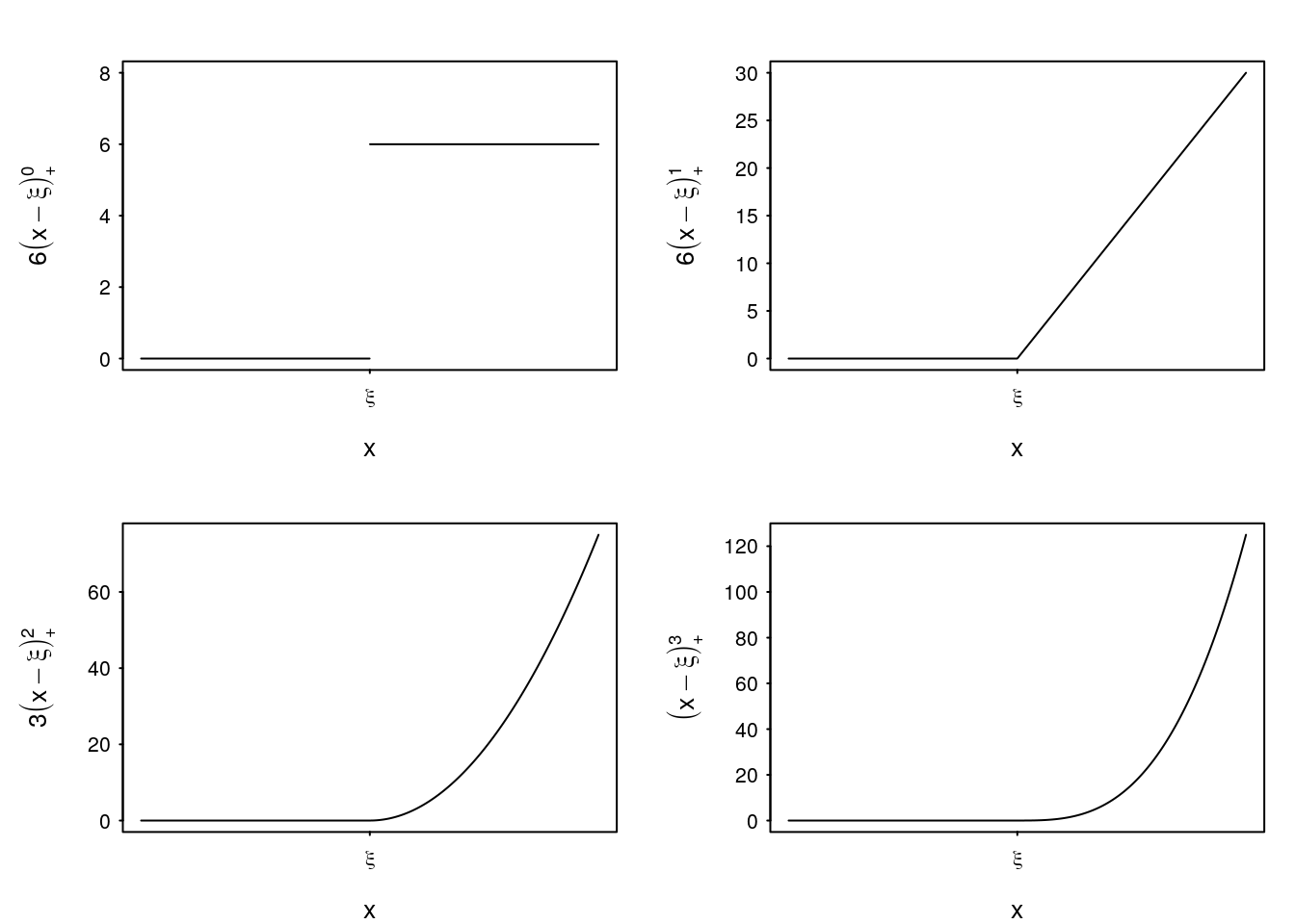
Figure 1: Example truncated power functions.
The TPB has stability issues as a basis. Therefore, alternatives are preferred. The \(k\)th-order B-spline basis can be defined as scaled \(k\)th divided differences of the TPB and any \(\Pi_{<k,\xi,\nu}\) has a B-spline basis.
For a function \(g\) and knot sequence \(\tau\), the \(k\)th divided difference of \(g\) is \[ [\tau_0,...,\tau_k]g = \begin{cases} \frac{g^{(k)}(\tau_0)}{k!} &\text{when }\tau_0=\tau_1=\cdots=\tau_k,g\in C^k \\ \frac{[\tau_0,...,\tau_{r-1},\tau_{r+1},...,\tau_k]g-[\tau_0,...,\tau_{s-1},\tau_{s+1},...,\tau_k]g}{t_s - t_r} &\text{where } t_s\text{ and }t_r\text{ are any distinct knots in the sequence.} \end{cases} \]
Let \(\tau = (\tau_j)\) be a nondecreasing sequence. The \(j\)th normalised B-spline of order \(k\) for the knot sequence \(\tau\), denoted \(B_{j,k,\tau}\) is \[ \begin{aligned} B_{j,k,\tau}(x) &\overset{\Delta}{=} (\tau_{j+k} - \tau_j)[\tau_j,...,\tau_{j+k}](\cdot - x)_+^{k-1} \\ &= [\tau_{j+1},...,\tau_{j+k}](\cdot - x)_+^{k-1} - [\tau_j,...,\tau_{j+k-1}](\cdot - x)_+^{k-1} \end{aligned} \] where the \(k\)th divided difference of \(g(\cdot)=(\cdot - x)_+^{k-1}\) is to be considered as a function of the knot for fixed \(x\). From the definition, if \(x\notin [\tau_j, \tau_{j+k})\) then \(B_{j,k,\tau}=0\).
Let \(\tau\) be a knot sequence. Then we have \[ B_{j1}(x) = \begin{cases} 1 &\text{if } x\in [\tau_j, \tau_{j+1}) \\ 0 & \text{if } x\notin [\tau_j, \tau_{j+1}) \end{cases} \] the B-spline of order 1. From this, the B-spline of order \(k>1\) on \([\tau_j, \tau_{j+k})\) are given by \[ \begin{aligned} B_{j,k}(x) &= \omega_{j,k}B_{j,k-1}(x) + (1 - \omega_{j+1,k})B_{j+1,k-1}(x) \\ &= \frac{x - \tau_j}{\tau_{j+k-1} - \tau_j}B_{j,k-1}(x) + \frac{\tau_{j+k} - x}{\tau_{j+k} - \tau_{j+1}}B_{j+1,k-1}(x) \\ \omega_{j,k}(x) &= \frac{x-\tau_j}{\tau_{j+k-1} - \tau_j} \end{aligned} \] which depends only on the \(k+1\) knots \(\tau_j,...,\tau_{j+k}\).
A spline function of order \(k\) with knot sequence \(\tau\) is any linear combination of B-splines of order \(k\) \[ \mathcal{S}_{k,\tau} \overset{\Delta}{=} \left\{\sum_i \alpha_i B_{i,k,\tau}|\alpha_i\in\mathbb R, \forall i\right\}. \] Given B-splines are in the set \(\Pi_{<k,\tau}\) we have \(\mathcal{S}_{k,\tau} \subseteq \Pi_{<k,\tau}\), but we also have \(\mathcal{S}_{k,\tau} = \Pi_{<k,\xi,\nu}\) for some \(\tau\) given \(\xi\) and \(\nu\). Additionally, \(\Pi_{<k}\subseteq \mathcal{S}_{k,\tau}\), that is, the set of splines contains all polynomials of order \(k\).
Curry and Schoenberg show that, given strictly increase break sequence \(\xi = (\xi_i)_1^{l+1}\), and non-negative integers \(\nu = (\nu_i)_2^l\) with \(\nu_i \leq k\), set \[ n \overset{\Delta}{=} k + \sum_{i=2}^l (k - \nu_i) = kl - \sum_{i=2}^l \nu_i = \dim\Pi_{<k,\xi,\nu} \] and let \(\tau = (\tau_i)_1^{n+k}\) be non-decreasing sequence constructed from \(xi\) and \(\nu\) by:
- for \(i=2,...,l\), \(\xi_i\) occurs exactly \(k-\nu_i\) times,
- \(\tau_1\leq \tau_2 \leq \cdots \leq \tau_k \leq \xi_1\) and \(\xi_{l+1}\leq \tau_{n+1} \leq \tau_{n+1} \leq \cdots \leq \tau_{n+k}\). Then the sequence \(B_1,...,B_n\) of B-splines of order \(k\) for knot sequence \(\tau\) is a basis for \(\Pi_{<k,\xi,\nu}\) as functions on the basic interval \(I_{k,\tau} = [\tau_k,...,\tau_{n+1}]\). This implies \[ \mathcal{S}_{k,\tau} = \Pi_{<k,\xi,nu} \text{ on } I_{k,\tau}. \] Thus, we have a recipe for constructing a B-spline basis for a piecewise polynomial space \(\Pi_{<k,\xi,\nu}\) by setting a certain knot sequence \(\tau\).
Fewer knots at a break \(\xi\) implies more continuity. The number of continuity conditions at a break plus the number of knots at the break is equal to the order of the spline. Additionally, \(k\)-knots at a break implies no continuity, and \(0\)-knots at a break implies \(k\) continuity conditions.
Summary
Truncated Power Basis
B-spline basis
M-spline basis
I-spline basis
Monotone Splines in Proportional Hazards Model
library(splines)
library(splines2)

knot_sequence <- function(breaks, continuity, order) {
  stopifnot(length(breaks) == length(continuity) + 2)
  stopifnot(all(continuity <= order))
  l <- length(breaks)

  n <- order + sum(order - continuity)
  c(rep(breaks[1], order),
    rep(breaks[2:(l-1)], times = order - continuity),
    rep(breaks[l], order))
}

build_b_spline <- function(x, knots, ind, order) {
    if(order == 1) {
      for (i in 1:size(t))
      b_spline[i] = (knots[ind] <= t[i]) && (t[i] < knots[ind + 1])
    } else {

    }
}
functions {
// B-spline construction (http://mc-stan.org/users/documentation/case-studies/splines_in_stan.html)
vector build_b_spline(real[] t, real[] knots, int ind, int order);
// INPUTS:
// t: the points at which the b_spline is calculated
// ext_knots: the set of extended knots
// ind: the index of the b_spline
// order: the order of the b-spline
vector build_b_spline(real[] t, real[] knots, int ind, int order) {
vector[size(t)] b_spline;
vector[size(t)] w1 = rep_vector(0, size(t));
vector[size(t)] w2 = rep_vector(0, size(t));
if (order == 1)
for (i in 1:size(t)) // B-splines of order 1 are piece-wise constant
b_spline[i] = (knots[ind] <= t[i]) && (t[i] < knots[ind + 1]);
else {
if (knots[ind] != knots[ind + order - 1])
w1 = (to_vector(t) - rep_vector(knots[ind], size(t))) /
(knots[ind + order - 1] - knots[ind]);
if (knots[ind+1] != knots[ind+order])
w2 = 1 - (to_vector(t) - rep_vector(knots[ind+1], size(t))) /
(knots[ind+order] - knots[ind+1]);
// Calculating the B-spline recursively as linear interpolation of two lower-order splines
b_spline = w1 .* build_b_spline(t, knots, ind, order - 1) +
w2 .* build_b_spline(t, knots, ind + 1, order - 1);
if (ind == size(knots) - order) {
b_spline[size(t)] = 1.0;
}
}
return b_spline;
}
// M-spline construction
vector build_m_spline(real[] t, real[] knots, int ind, int order);
// INPUTS
// t: points at which to calculate M-spline
// ext_knots: set of extended knots
// ind: index of M spline
// order: order of M spline
vector build_m_spline(real[] t, real[] knots, int ind, int order) {
vector[size(t)] b_spline;
vector[size(t)] m_spline;
b_spline = build_b_spline(t, knots, ind, order);
for (i in 1:size(t)) {
m_spline[i] = b_spline[i]*order/(knots[ind + order] - knots[ind]);
}
return m_spline;
}
// I-spline construction
matrix b_spline_to_i_spline(matrix B);
// INPUTS
// B: a bSpline of degree k + 1
// will produce an iSpline of degree k
matrix b_spline_to_i_spline(matrix B) {
int dim[2];
row_vector[dims(B)[2]] rev_b;
matrix[dims(B)[1], dims(B)[2]] i_spline;
for(i in 1:dims(B)[1]) {
i_spline[i] = to_row_vector(rep_vector(0, dims(B)[2]));
// need to reverse, cumulative sum, then reverse again.
// better way to do it? reverse(x) function?
for(j in 1:dims(B)[2]) {
rev_b[j] = B[i][dims(B)[2] - j + 1];
}
rev_b = cumulative_sum(rev_b);
for(j in 1:dims(B)[2]) {
i_spline[i, j] = rev_b[dims(B)[2] - j + 1];
}
}
return i_spline;
}
}Examples
library(simsurv)
covs <- data.frame(id = 1:1000, trt = factor(sample.int(3, 1000, replace = T)))
X <- data.frame(cbind(covs, model.matrix( ~ trt, data = covs)[, -1]))
sim <- simsurv(lambdas = 0.2, gammas = 1.5, betas = c(trt2 = 0),
               x = X, tde = c(trt2 = 0.5), tdefunction = function(x) (x > 2))
plot(ecdf(sim$eventtime[X$trt2 == 0]))
lines(ecdf(sim$eventtime[X$trt2 == 1]), col = "red")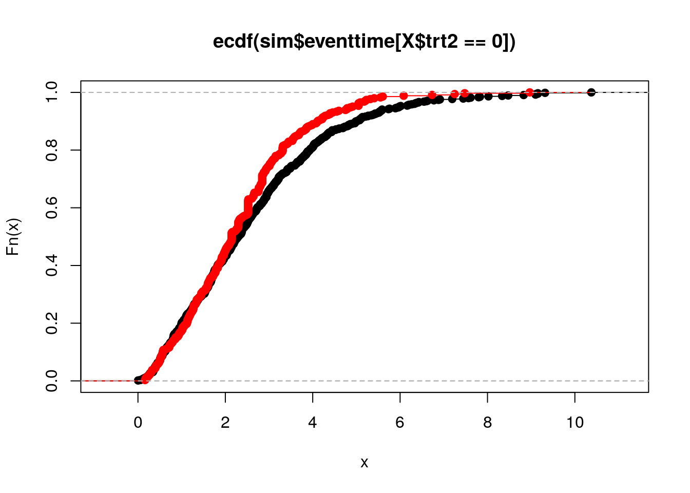
References
De Boor, Carl. 1978. A Practical Guide to Splines. Vol. 27. springer-verlag New York.
Ramsay, James O, and others. 1988. “Monotone Regression Splines in Action.” Statistical Science 3 (4): 425–41.