Variational Approximations
Variational Bayes is an approximate Bayesian inference method based on choosing an approximating density from some restricted class of densities by minimising the Kullback-Leibler divergence \[ \text{KL}(p\vert\vert q) = \int_\Omega \log\frac{p(\theta)}{q(\theta)} p(\theta)d\theta. \] In Bayesian inference, the density to be approximated is usually the posterior probability of some model parameter of interest \[ p(\theta|y) = \frac{p(\theta,y)}{p(y )}, \] and so the approximating density \(q\) is chosen as \[ q^\star(\theta) = \underset{q\in\mathcal{Q}}{\text{argmin }} \text{KL}(q\lvert\rvert p). \] It can be shown (Ormerod and Wand 2010) that minimising the Kullback-Leibler divergence is equivalent to maximising a lower bound on the marginal likelihood \[ \begin{aligned} q^\star(\theta) &= \underset{q\in\mathcal{Q}}{\text{argmax }}\mathcal{L}(q) \\ \mathcal{L}(q) &= \exp\left\{\int_\Omega \ln\left[\frac{p(y,\theta)}{q(\theta)}\right] q(\theta)d\theta\right\} \end{aligned} \] Expanding the above we have \[ \begin{aligned} \ln \mathcal{L}(q) &= \mathbb E_q[\ln p(y|\theta)] + \mathbb E_q[\ln p(\theta)] - \mathbb E_q[\ln q(\theta)] \\ &= \mathbb E_q[\ln p(y|\theta)] + \mathbb E_q[\ln p(\theta)] + \mathbb H[q] \end{aligned} \] where \(\mathbb H[q]\) denotes the entropy of \(q\).
Rhode and Wand (2016) delineate between three class of variational approximation: parametric, nonparametric, and semiparametric.
In parametric variational Bayes, the approximating class is restricted to some parametric family \[ \mathcal{Q} = \{q(\theta;\xi)|\xi\in\Xi\}. \] In nonparametric variational Bayes, where the approximating class is not specified to belong to some parametric family, but only that it be factored into independent components (also known as mean-field variational Bayes) \[ \mathcal{Q} = \{q(\theta)|q(\theta) = q_1(\theta_1)\cdots q_M(\theta_M)\}. \] Semiparametric variational Bayes is a compromise between the two, where some parts of the parameter space are constrained to have a specific parametric form, but others are unspecified \[ \mathcal{Q} = \{q(\theta)|q(\theta) = q(\theta_0;\xi)q_1(\theta_1)\cdots q_M(\theta_M),\xi\in\Xi\}. \]
Combining solutions to the parametric and nonparametric cases, (Rhode and Wand 2016, Algorithm 1) the general approach to optimising the \(q\)-densities is given in Proposition 1.Proposition 1 (Algorithm to optimise semiparametric variational Bayes density) Initialise: \(q(\theta_1)\cdots q(\theta_M)\)
Cycle: \[ \begin{aligned} \xi &\leftarrow \underset{\xi^\prime\in\Xi}{\text{argmax }} \left\{\ln \mathcal{L}(q,\xi^\prime)^{[\theta_0]}\right\} \\ q(\theta_1) &\leftarrow \frac{\exp\left\{\mathbb E_{q(\theta_{-1})}[\ln p(y,\theta)]\right\}}{\int \exp\left\{\mathbb E_{q(\theta_{-1})}[\ln p(y,\theta)]\right\}d\theta_1} \\ &\vdots \\ q(\theta_M) &\leftarrow \frac{\exp\left\{\mathbb E_{q(\theta_{-M})}[\ln p(y,\theta)]\right\}}{\int \exp\left\{\mathbb E_{q(\theta_{-M})}[\ln p(y,\theta)]\right\}d\theta_M} \end{aligned} \] unti convergence of \(\mathcal{L}(q,\xi)\).In Proposition 1, \(\mathcal{L}(q,\xi^\prime)^{[\theta_0]}\) is the \(\theta_0\)-localised component of the marginal likelihood lower bound.
Further, if one specifies \(q(\theta_0;\xi) = N(\theta_0;\mu_q, \Sigma_q)\) then the optimisation scheme in step one follows the natural fixed-point iterations given in Proposition 2 (Rhode and Wand 2016, Result 2).Exponential Proportional Hazards Model
As an exercise, I now apply the above results to the parametric proportional hazards model assuming exponential density (constant hazard) and right-censoring. Suppose we specify an exponential regression model \(f(y_i) = \exp(x_i^\top\beta)\) where \(\beta_0 = \ln\lambda\) the baseline hazard.
Suppose that \(y_{1:n}\) are survival times subject to right-censoring as indicated by \(\nu_{1:n}\). We specify the model the complete model \[ \begin{aligned} p(\beta) &= N(\theta|\mu_0,\Sigma_0) \\ \ln p(\beta) &= -\frac{d}{2}\ln(2\pi) - \frac{1}{2}\ln|\Sigma_0| - \frac{1}{2}(\beta - \mu_0)^\top\Sigma_0^{-1}(\beta-\mu_0)\\ p(y_i|\beta;\nu_{1:n}) &= \prod_{i=1}^n \exp(x_i^\top\beta)^{\nu_i}\exp(-y_i\exp(x_i^\top\beta))\\ \ln p(y|\beta;\nu) &= v^\top X\beta - y^\top\exp(X\beta) \\ \ln p(\beta|y;\nu) &= k+v^\top X\beta - y^\top\exp(X\beta) -\frac{1}{2}\ln|\Sigma_0| - \frac{1}{2}(\beta - \mu_0)^\top\Sigma_0^{-1}(\beta-\mu_0) \end{aligned} \] for some constant \(k\).
Suppose we specify the approximating class \(\mathcal{Q} = \{q(\beta)|q(\beta;\xi) = N(\beta|\mu_\beta,\Sigma_\beta)\}\), then this is parametric variational inference. We know the multivariate normal distribution has entropy \[ \mathbb H[q] = \frac{1}{2}d[1 + \ln(2\pi)] + \frac{1}{2}\ln|\Sigma_q|. \]
Also, \[ \begin{aligned} \mathbb E_q[\ln p(\beta)] &= -\frac{d}{2}\ln(2\pi) -\frac{1}{2}|\Sigma_0| - \frac{1}{2}\mathbb E_q[(\beta-\mu_0)^\top\Sigma_0^{-1}(\beta-\mu_0)] \\ &= -\frac{d}{2}\ln(2\pi) -\frac{1}{2}|\Sigma_0| - \frac{1}{2}\mathbb E_q[\beta-\mu_0]^\top\Sigma_0^{-1}\mathbb E[\beta-\mu_0] - \frac{1}{2}\text{tr}\left[\Sigma_0^{-1}\mathbb V_q(\beta-\mu_0)\right] \\ &= -\frac{d}{2}\ln(2\pi) -\frac{1}{2}|\Sigma_0| - \frac{1}{2}(\mu_q-\mu_0)^\top\Sigma_0^{-1}(\mu_q-\mu_0) - \text{tr}(\Sigma_0^{-1}\Sigma_q) \end{aligned} \] where we have used the fact \(\mathbb E[X^\top A X] = \mu^\top A\mu + \text{tr}(A\Sigma)\).
Finally, \[ \begin{aligned} \mathbb E_q[\ln p(y|\beta;\nu)] &= \nu^\top X\mathbb E_q[\beta] - y^\top\mathbb E_q[e^{X\beta}] \\ &= \nu^\top X\mu_q - y^\top e^{X\mu_q + \text{diag}(X\Sigma_q X^\top)/2} \end{aligned} \] using the fact that if \(X\sim N(\mu, \Sigma)\) then \(\mathbb E[e^X] = e^{\mu + \text{diag}(\Sigma)/2}\).
To obtain the fixed-point updates we need to differentiate the relevant expressions. \[ \begin{aligned} \mathsf{D}_{\mu_q}\left(\mathcal{L}(q;\mu_q,\Sigma_q)^{[\beta]}\right) &= \nu^\top X-y^\top e^{X\mu_q + \text{diag}(X\Sigma_q X^\top)/2}X - \Sigma_0^{-1}(\mu_q - \mu_0) \\ &= X^\top\left(\nu - y\odot e^{X\mu_q + \text{diag}(X\Sigma_0 X^\top)/2}\right) - \Sigma_0^{-1}(\mu_q - \mu_0)\\ \mathsf{H}_{\mu_q}\left(\mathcal{L}(q;\mu_q,\Sigma_q)^{[\beta]}\right) &= -X^\top\text{diag}\left(y\odot e^{X\mu_q + \text{diag}(X\Sigma_0 X^\top)/2}\right)X - \Sigma_0^{-1}. \end{aligned} \] Now we have the fixed-point updates to find \(\underset{\xi\in \Xi}{\text{argmax }} \mathcal{L}(q;\mu_q,\Sigma_q)\) \[ \begin{cases} \omega_q \leftarrow y \odot e^{X\mu_q + \text{diag}(X\Sigma_q X)/2}\\ \Sigma_q \leftarrow \left(X^\top\text{diag}(\omega_q)X + \Sigma_0^{-1}\right)^{-1}\\ \mu_q \leftarrow \mu_q + \Sigma_q\left(X^\top(\nu - \omega_q) - \Sigma_0^{-1}(\mu_q - \mu_0)\right). \end{cases} \]
Example
The above algorithm is implemented below and compared to results from estimation of the same model in Stan.
# Entropy for multivariate normal
mvn_ent <- function(Sigma) {
  (ncol(Sigma)*(1 + log(2*pi)) + log(det(Sigma)))/2
}

# VB for PH Exponential
ph_exp_vb <- function(X, y, v, mu0, Sigma0, maxiter = 100, tol = 1e-5, verbose = FALSE) {
  d <- ncol(X)
  invSigma0 <- solve(Sigma0)
  mu <- mu0
  Sigma <- Sigma0
  lb <- as.numeric(maxiter)
  i <- 0
  converged <- FALSE
  while(i <= maxiter & !converged) {
    i <- i + 1
    omega <- y * exp(X %*% mu + diag(tcrossprod(X %*% Sigma, X))/2)[, 1]
    Sigma <- solve(crossprod(X, diag(omega) %*% X) + invSigma0)
    mu <- mu + Sigma %*% (crossprod(X, v - omega) - invSigma0 %*% (mu - mu0))

    # Calculate L(q)
    Xmu <- X %*% mu
    lb[i] <- mvn_ent(Sigma) +
      crossprod(v, Xmu) - crossprod(y, exp(Xmu + diag(tcrossprod(X %*% Sigma, X))/2)) -
      d*log(det(Sigma0))/2 -
      crossprod(mu - mu0, invSigma0 %*% (mu - mu0))/2 -
      sum(diag(invSigma0 %*% Sigma))/2
    if(verbose) cat("Iteration ", i, "ELBO = ", lb[i], "\n")
    if(i > 1 && abs(lb[i] - lb[i - 1]) < tol) converged <- TRUE
  }
  return(list(lb = lb[1:i], mu = mu, Sigma = Sigma))
}
// Stan model for PH Exponential (ph_exp_stan)
data {
int<lower=1> N;
int<lower=0> K;
vector[N] y;
int v[N];
matrix[N, K] X;
vector[K] mu0;
matrix[K, K] Sigma0;
}
parameters {
vector[K] beta;
}
model {
vector[N] eta = X*beta;
beta ~ multi_normal(mu0, Sigma0);
for(n in 1:N) {
if (v[n] == 1)
y[n] ~ exponential(exp(eta[n]));
else
target += exponential_lccdf(y[n] | exp(eta[n]));
}
}
library(rstan)
set.seed(4231)
X <- cbind(1, rep(c(0, 1), each = 100))
b <- c(log(1/35), 5)
y <- yu <- rexp(nrow(X), exp(X %*% b))
v <- 1 - as.numeric(yu > 15)
y[v == 0] <- 15
mu0 <- c(0, 0)
Sigma0 <- diag(2)

vb_fit <- ph_exp_vb(X, y, v, mu0, Sigma0, verbose = TRUE)
Iteration 1 ELBO = -484.1595
Iteration 2 ELBO = -237.9834
Iteration 3 ELBO = -153.1951
Iteration 4 ELBO = -139.9239
Iteration 5 ELBO = -139.0202
Iteration 6 ELBO = -139.0043
Iteration 7 ELBO = -139.0042
Iteration 8 ELBO = -139.0042 stan_fit <- sampling(ph_exp_stan,
data = list(X = X, y = y, v = v,
N = nrow(X), K = ncol(X),
mu0 = mu0, Sigma0 = Sigma0),
refresh = 0)par(mfrow = c(2, 2), cex = 0.75)
plot(1:length(vb_fit$lb), vb_fit$lb, xlab = "Iteration", ylab = "ELBO(q)", type = 'l')
title("a)", adj = 0)
plot(0, type = 'n', xaxt = 'n', yaxt = 'n', bty = 'n', pch = '', ylab = '', xlab = '')
hist(extract(stan_fit)$beta[, 1], prob = T, breaks = 50,
xlab = expression(beta[0]), main = "")
title("b)", adj = 0)
curve(dnorm(x, vb_fit$mu[1], sqrt(vb_fit$Sigma[1, 1])), add = TRUE)
hist(extract(stan_fit)$beta[, 2], prob = T, breaks = 50,
main = "", xlab = expression(beta[1]))
curve(dnorm(x, vb_fit$mu[2], sqrt(vb_fit$Sigma[2, 2])), add = TRUE)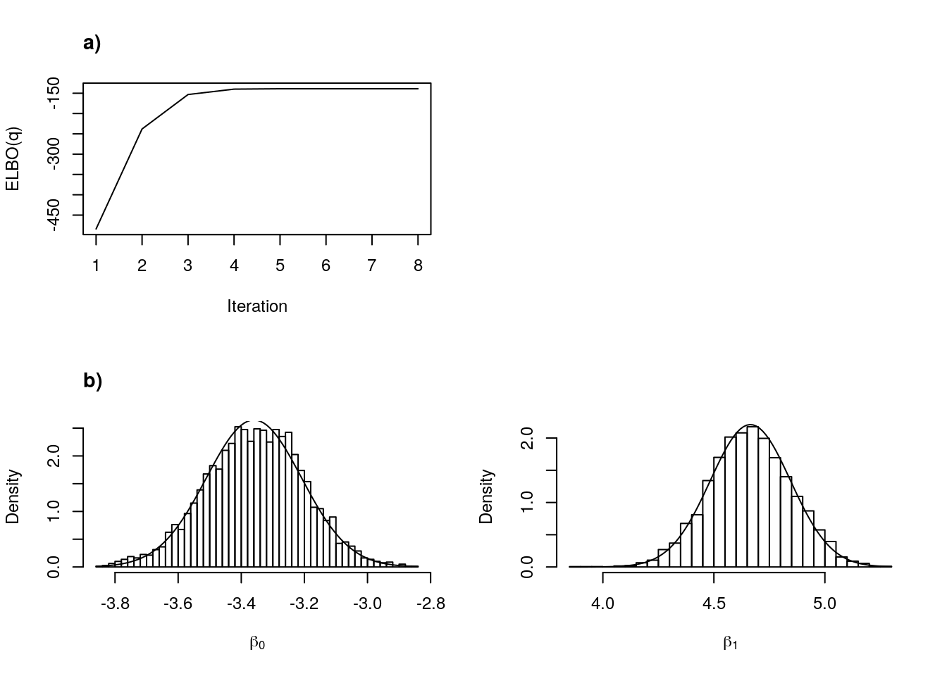
Figure 1: a) Convergence of VB, and b) comparison of variation approximation and dynamic HMC.
Summary
A variational approximation for the exponential proportional hazards model under right-censoring was derived following the results in Rhode and Wand (2016). For more complicated survival models the derivations are unlikely to be as straightforward, but it would be interesting to investigate for other cases.
References
Ormerod, John T., and Matt P. Wand. 2010. “Explaining Variational Approximations.” The American Statistician 64 (2): 140–53.
Rhode, David, and Matt P. Wand. 2016. “Semiparametric Mean Field Variational Bayes: General Principles and Numerical Issues.” Journal of Machine Learning Research 17: 1–47.